TableMage Demonstration
TableMage is a Python package for low-code/conversational data science. In this notebook, we provide a few examples of how the package can be used.
Notebook Contents
Introduction
Exploratory Data Analysis
Regression Analysis
Causal Inference
Machine Learning
Conversational Data Analysis
Section 1: Introduction
1.1: Installation
Let’s first install the package. On a local machine, you simply need to copy-and-paste the following code into your terminal:
git clone https://github.com/ajy25/TableMage.git
cd TableMage
pip install .
If you want to use the conversational data analysis mode, you should replace the last line with the following line:
pip install '.[agents]'
NOTE: If you are a MacOS user, you’ll need to install libomp. It’s a dependency for using XGBoost, a TableMage dependency.
Okay! Let’s run the cell below. On Google Colab, you’ll be prompted to restart the session—this is normal.
[1]:
using_google_colab = False
If using Colab, copy and paste the following code block into a cell below and run it.
%%capture
!pip uninstall -y tablemage
!rm -rf TableMage
!git clone https://github.com/ajy25/TableMage.git
%cd TableMage
!pip install '.[agents]'
[2]:
from pathlib import Path

project_dir = Path.cwd().parent.resolve()
import sys

sys.path.append(str(project_dir))
import tablemage as tm

print(tm.__description__)
Python package for low-code/conversational clinical data science.
1.2 The Analyzer Class
Now that TableMage is installed, let’s try importing the package. We’ll use a toy dataset from scikit-learn for now.
[3]:
from sklearn.datasets import load_breast_cancer
import pandas as pd

brca_dataset = load_breast_cancer()
df = pd.DataFrame(data=brca_dataset.data, columns=brca_dataset.feature_names)
df["target"] = brca_dataset.target
df.head()
[3]:
| mean radius | mean texture | mean perimeter | mean area | mean smoothness | mean compactness | mean concavity | mean concave points | mean symmetry | mean fractal dimension | ... | worst texture | worst perimeter | worst area | worst smoothness | worst compactness | worst concavity | worst concave points | worst symmetry | worst fractal dimension | target | |
|---|---|---|---|---|---|---|---|---|---|---|---|---|---|---|---|---|---|---|---|---|---|
| 0 | 17.99 | 10.38 | 122.80 | 1001.0 | 0.11840 | 0.27760 | 0.3001 | 0.14710 | 0.2419 | 0.07871 | ... | 17.33 | 184.60 | 2019.0 | 0.1622 | 0.6656 | 0.7119 | 0.2654 | 0.4601 | 0.11890 | 0 |
| 1 | 20.57 | 17.77 | 132.90 | 1326.0 | 0.08474 | 0.07864 | 0.0869 | 0.07017 | 0.1812 | 0.05667 | ... | 23.41 | 158.80 | 1956.0 | 0.1238 | 0.1866 | 0.2416 | 0.1860 | 0.2750 | 0.08902 | 0 |
| 2 | 19.69 | 21.25 | 130.00 | 1203.0 | 0.10960 | 0.15990 | 0.1974 | 0.12790 | 0.2069 | 0.05999 | ... | 25.53 | 152.50 | 1709.0 | 0.1444 | 0.4245 | 0.4504 | 0.2430 | 0.3613 | 0.08758 | 0 |
| 3 | 11.42 | 20.38 | 77.58 | 386.1 | 0.14250 | 0.28390 | 0.2414 | 0.10520 | 0.2597 | 0.09744 | ... | 26.50 | 98.87 | 567.7 | 0.2098 | 0.8663 | 0.6869 | 0.2575 | 0.6638 | 0.17300 | 0 |
| 4 | 20.29 | 14.34 | 135.10 | 1297.0 | 0.10030 | 0.13280 | 0.1980 | 0.10430 | 0.1809 | 0.05883 | ... | 16.67 | 152.20 | 1575.0 | 0.1374 | 0.2050 | 0.4000 | 0.1625 | 0.2364 | 0.07678 | 0 |
5 rows × 31 columns
The Analyzer is the bridge between the data and the analysis methods. Most likely, you’ll want to do some modeling of some sort, such as linear regression or some type of machine learning regression/classification. As such, the Analyzer splits the data into a train dataset and a withheld test dataset upon initialization.
Be careful! The Analyzer will rename variables to make them easily formula-compatible (i.e., replace spaces and other prohibited characters with underscores). It is recommended that you remove spaces and special characters from variable names before you initialize an Analyzer, just to make sure you have full control over the names. A good rule-of-thumb is to avoid punctuation and spaces, with the exceptions of “_” and “.”, which are totally fine. We’ll let Analyzer handle the renaming for now.
[4]:
analyzer = tm.Analyzer(
    df, test_size=0.2, split_seed=42, verbose=True, name="Breast Cancer"
)

# You can also split the dataset yourself, e.g. ...
# df_train, df_test = sklearn.train_test_split(df, random_state=42)
# analyzer = tm.Analyzer(df_train, df_test=df_test)
UPDT: Renamed variables 'area error', 'compactness error', 'concave points error',
      'concavity error', 'fractal dimension error', 'mean area', 'mean compactness',
      'mean concave points', 'mean concavity', 'mean fractal dimension', 'mean
      perimeter', 'mean radius', 'mean smoothness', 'mean symmetry', 'mean texture',
      'perimeter error', 'radius error', 'smoothness error', 'symmetry error', 'texture
      error', 'worst area', 'worst compactness', 'worst concave points', 'worst
      concavity', 'worst fractal dimension', 'worst perimeter', 'worst radius', 'worst
      smoothness', 'worst symmetry', 'worst texture' to 'area_error',
      'compactness_error', 'concave_points_error', 'concavity_error',
      'fractal_dimension_error', 'mean_area', 'mean_compactness', 'mean_concave_points',
      'mean_concavity', 'mean_fractal_dimension', 'mean_perimeter', 'mean_radius',
      'mean_smoothness', 'mean_symmetry', 'mean_texture', 'perimeter_error',
      'radius_error', 'smoothness_error', 'symmetry_error', 'texture_error',
      'worst_area', 'worst_compactness', 'worst_concave_points', 'worst_concavity',
      'worst_fractal_dimension', 'worst_perimeter', 'worst_radius', 'worst_smoothness',
      'worst_symmetry', 'worst_texture'.
UPDT: Analyzer initialized for dataset 'Breast Cancer'.
TableMage is designed for notebooks. Many objects are display-friendly!
[5]:
analyzer
[5]:
========================================================================================
Breast Cancer
----------------------------------------------------------------------------------------
Train shape: (455, 31)                      Test shape: (114, 31)
----------------------------------------------------------------------------------------
Categorical variables:
  None

Numeric variables:
  'area_error', 'compactness_error', 'concave_points_error', 'concavity_error',
  'fractal_dimension_error', 'mean_area', 'mean_compactness', 'mean_concave_points',
  'mean_concavity', 'mean_fractal_dimension', 'mean_perimeter', 'mean_radius',
  'mean_smoothness', 'mean_symmetry', 'mean_texture', 'perimeter_error', 'radius_error',
  'smoothness_error', 'symmetry_error', 'target', 'texture_error', 'worst_area',
  'worst_compactness', 'worst_concave_points', 'worst_concavity',
  'worst_fractal_dimension', 'worst_perimeter', 'worst_radius', 'worst_smoothness',
  'worst_symmetry', 'worst_texture'
========================================================================================
Before we proceed, let’s discuss why TableMage requires train-test splitting upon initialization. TableMage aims to accelerate data science on tabular data. Often, the end goal is to train a model to predict a target, such as whether or not a patient has breast cancer based on geometrical features, or a patient’s billing amoung given the health insurer and disease type. In these cases, it is incredibly important to think in terms of pipelines, especially when transformations must be made to the data. Transformations—including missing data imputation and feature scaling—must be “fit” on the train data only. Performing data transformations based on the entire dataset is a common mistake, even for experienced data scientists.
TableMage handles all of this for you. You can explore the dataset (looking at the entire dataset or only the train or test dataset—your choice), make transformations such as imputation, feature engineering, and scaling, and immediately train a model to predict a target variable, without needing to worry about all the intermediate details! Hopefully, this will be more clear in section 5, when we discuss machine learning.
If you don’t plan on doing any modeling, simply set test_size to 0.
1.3 Submodules
TableMage has two submodules:
ml: Machine learning models
fs: Feature selection models
Let’s print an object from each. These will be discussed in greater detail in section 5.
[6]:
print(tm.ml.LinearC())
print(tm.fs.BorutaFSR())
LinearC(l2)
BorutaFSR
Section 2: Exploratory Data Analysis
Let’s explore a dataset. We’ll use the Kaggle House Prices dataset as an example since it contains a good amount of categorical and numeric features with varying levels of missingness.
[7]:
from pathlib import Path
import matplotlib.pyplot as plt

plt.rcParams["figure.dpi"] = 150

if using_google_colab:
    curr_dir = Path.cwd()
else:
    curr_dir = Path("__notebook__").resolve().parent

data_path = curr_dir.parent / "demo" / "regression" / "house_price_data" / "data.csv"
df = pd.read_csv(data_path, index_col=0)
analyzer = tm.Analyzer(
    df, test_size=0.2, split_seed=42, verbose=True, name="House Prices"
)
analyzer
UPDT: Analyzer initialized for dataset 'House Prices'.
[7]:
========================================================================================
House Prices
----------------------------------------------------------------------------------------
Train shape: (1168, 80)                      Test shape: (292, 80)
----------------------------------------------------------------------------------------
Categorical variables:
  'Alley', 'BldgType', 'BsmtCond', 'BsmtExposure', 'BsmtFinType1', 'BsmtFinType2',
  'BsmtQual', 'CentralAir', 'Condition1', 'Condition2', 'Electrical', 'ExterCond',
  'ExterQual', 'Exterior1st', 'Exterior2nd', 'Fence', 'FireplaceQu', 'Foundation',
  'Functional', 'GarageCond', 'GarageFinish', 'GarageQual', 'GarageType', 'Heating',
  'HeatingQC', 'HouseStyle', 'KitchenQual', 'LandContour', 'LandSlope', 'LotConfig',
  'LotShape', 'MSZoning', 'MasVnrType', 'MiscFeature', 'Neighborhood', 'PavedDrive',
  'PoolQC', 'RoofMatl', 'RoofStyle', 'SaleCondition', 'SaleType', 'Street', 'Utilities'

Numeric variables:
  '1stFlrSF', '2ndFlrSF', '3SsnPorch', 'BedroomAbvGr', 'BsmtFinSF1', 'BsmtFinSF2',
  'BsmtFullBath', 'BsmtHalfBath', 'BsmtUnfSF', 'EnclosedPorch', 'Fireplaces',
  'FullBath', 'GarageArea', 'GarageCars', 'GarageYrBlt', 'GrLivArea', 'HalfBath',
  'KitchenAbvGr', 'LotArea', 'LotFrontage', 'LowQualFinSF', 'MSSubClass', 'MasVnrArea',
  'MiscVal', 'MoSold', 'OpenPorchSF', 'OverallCond', 'OverallQual', 'PoolArea',
  'SalePrice', 'ScreenPorch', 'TotRmsAbvGrd', 'TotalBsmtSF', 'WoodDeckSF', 'YearBuilt',
  'YearRemodAdd', 'YrSold'
========================================================================================
2.1 Plots
We can begin our analysis by using TableMage to make plots of the dataset.
[8]:
analyzer.eda().plot("SalePrice")
[8]:
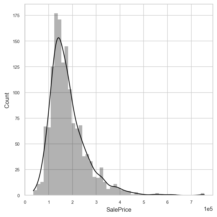
By default, Analyzer considers the entire dataset (train and test) for exploratory analysis. You can change this by specifying which dataset you would like to consider in the analyzer.eda() method.
[9]:
analyzer.eda("train").plot("SalePrice")
[9]:
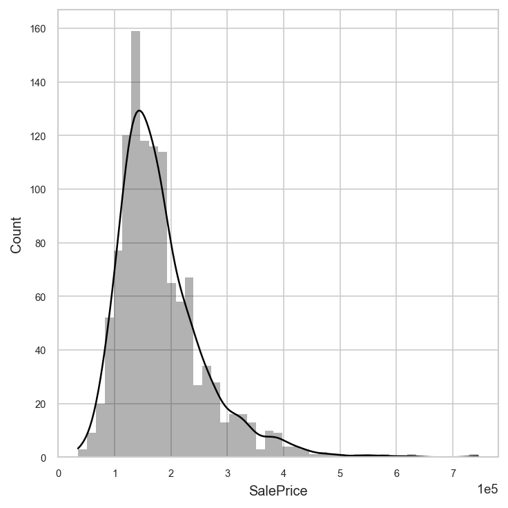
Let’s plot the sale price versus 1st floor square footage.
[10]:
analyzer.eda().plot("SalePrice", "1stFlrSF")
[10]:
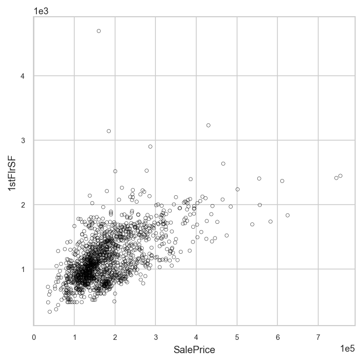
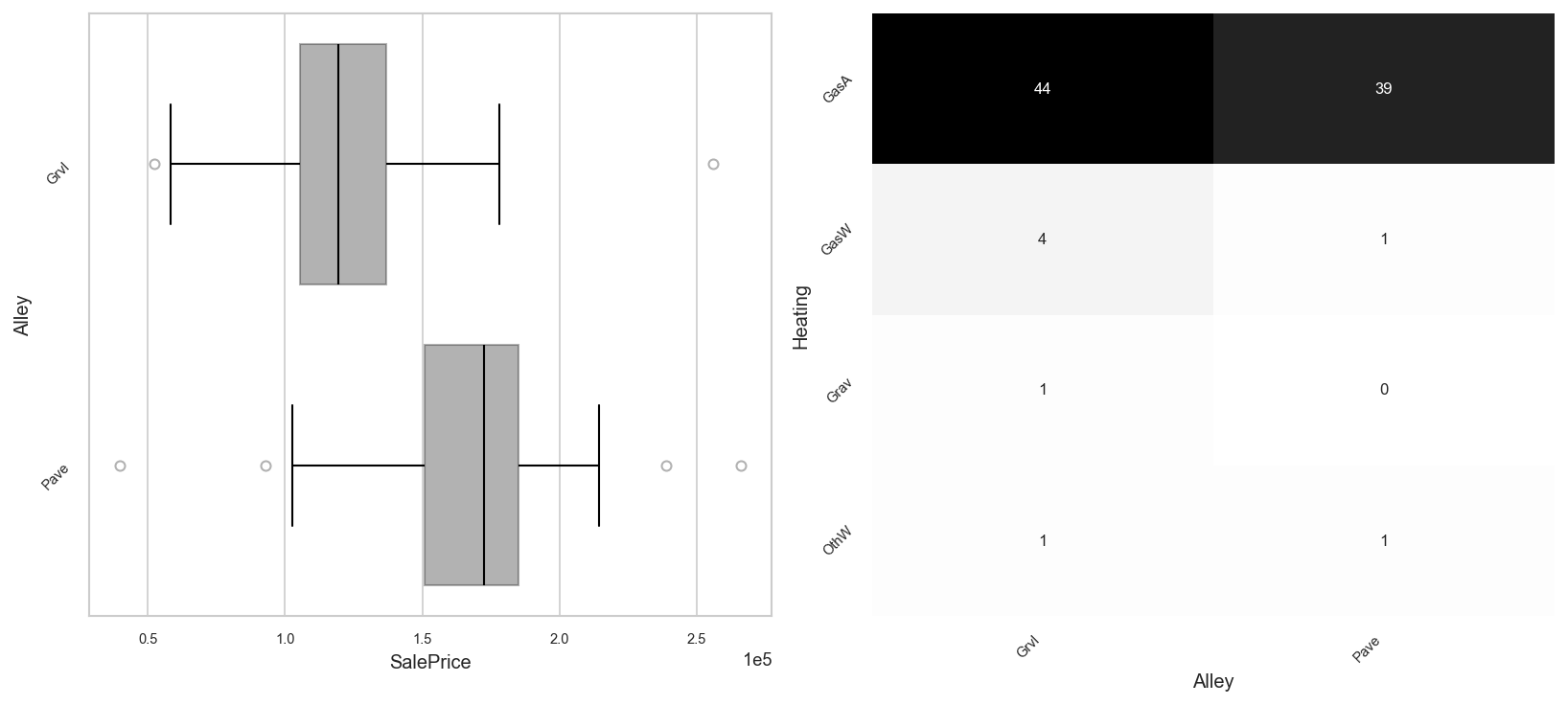
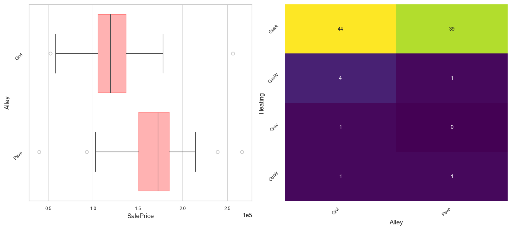
You can plot any two variables agains each other, regardless of whether they are numeric or categorical.
[11]:
fig, axs = plt.subplots(ncols=2, figsize=(11, 5))
analyzer.eda().plot("SalePrice", "Alley", ax=axs[0])
analyzer.eda().plot("Alley", "Heating", ax=axs[1])
[11]:
You can change colors.
[12]:
tm.options.plot_options.set_color_map("viridis")
tm.options.plot_options.set_bar_color("red")
fig, axs = plt.subplots(ncols=2, figsize=(11, 5))
analyzer.eda().plot("SalePrice", "Alley", ax=axs[0])
analyzer.eda().plot("Alley", "Heating", ax=axs[1])
[12]:
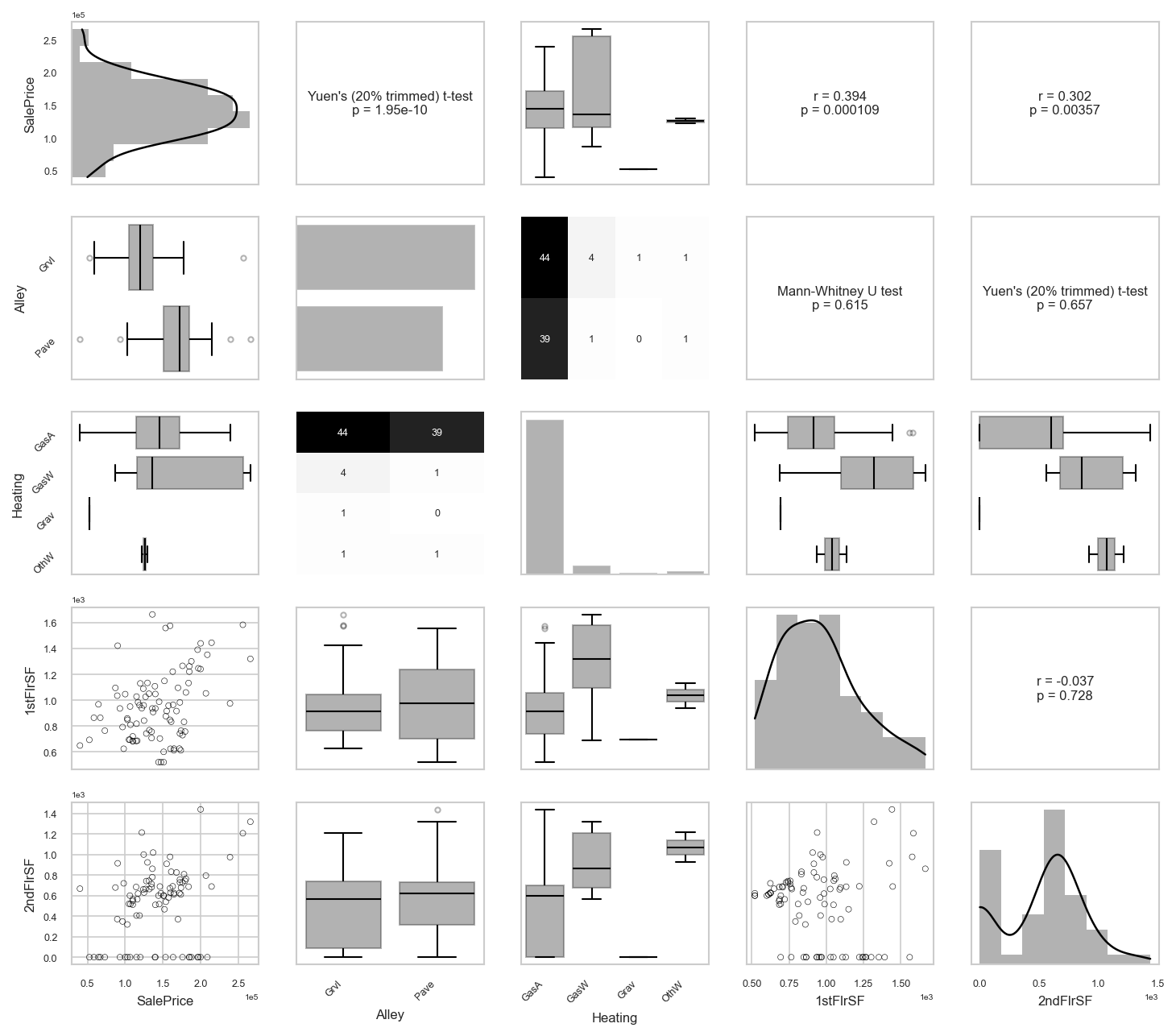
You can make pair plots, like in R. Hypothesis tests are automatically selected based on data normality and homoskedasticity
[13]:
tm.options.plot_options.set_to_defaults()
tm.options.plot_options.set_font_sizes(
    axis_title=8, major_ticklabel=6, minor_ticklabel=5
)
analyzer.eda().plot_pairs(
    ["SalePrice", "Alley", "Heating", "1stFlrSF", "2ndFlrSF"],
    htest=True,
    figsize=(10, 10),
)
[13]:
2.2 Tables
We can display all the basic statistics of each numerical variable.
[14]:
analyzer.eda().numeric_stats()
[14]:
| Statistic | min | max | mean | std | variance | skew | kurtosis | q1 | median | q3 | n_missing | missing_rate | n |
|---|---|---|---|---|---|---|---|---|---|---|---|---|---|
| Variable | |||||||||||||
| 1stFlrSF | 334.0 | 4692.0 | 1162.627 | 386.588 | 1.494501e+05 | 1.375 | 5.722 | 882.00 | 1087.0 | 1391.25 | 0 | 0.000 | 1460 |
| 2ndFlrSF | 0.0 | 2065.0 | 346.992 | 436.528 | 1.905571e+05 | 0.812 | -0.556 | 0.00 | 0.0 | 728.00 | 0 | 0.000 | 1460 |
| 3SsnPorch | 0.0 | 508.0 | 3.410 | 29.317 | 8.595060e+02 | 10.294 | 123.235 | 0.00 | 0.0 | 0.00 | 0 | 0.000 | 1460 |
| BedroomAbvGr | 0.0 | 8.0 | 2.866 | 0.816 | 6.650000e-01 | 0.212 | 2.219 | 2.00 | 3.0 | 3.00 | 0 | 0.000 | 1460 |
| BsmtFinSF1 | 0.0 | 5644.0 | 443.640 | 456.098 | 2.080255e+05 | 1.684 | 11.076 | 0.00 | 383.5 | 712.25 | 0 | 0.000 | 1460 |
| BsmtFinSF2 | 0.0 | 1474.0 | 46.549 | 161.319 | 2.602391e+04 | 4.251 | 20.040 | 0.00 | 0.0 | 0.00 | 0 | 0.000 | 1460 |
| BsmtFullBath | 0.0 | 3.0 | 0.425 | 0.519 | 2.690000e-01 | 0.595 | -0.840 | 0.00 | 0.0 | 1.00 | 0 | 0.000 | 1460 |
| BsmtHalfBath | 0.0 | 2.0 | 0.058 | 0.239 | 5.700000e-02 | 4.099 | 16.336 | 0.00 | 0.0 | 0.00 | 0 | 0.000 | 1460 |
| BsmtUnfSF | 0.0 | 2336.0 | 567.240 | 441.867 | 1.952464e+05 | 0.919 | 0.469 | 223.00 | 477.5 | 808.00 | 0 | 0.000 | 1460 |
| EnclosedPorch | 0.0 | 552.0 | 21.954 | 61.119 | 3.735550e+03 | 3.087 | 10.391 | 0.00 | 0.0 | 0.00 | 0 | 0.000 | 1460 |
| Fireplaces | 0.0 | 3.0 | 0.613 | 0.645 | 4.160000e-01 | 0.649 | -0.221 | 0.00 | 1.0 | 1.00 | 0 | 0.000 | 1460 |
| FullBath | 0.0 | 3.0 | 1.565 | 0.551 | 3.040000e-01 | 0.037 | -0.858 | 1.00 | 2.0 | 2.00 | 0 | 0.000 | 1460 |
| GarageArea | 0.0 | 1418.0 | 472.980 | 213.805 | 4.571251e+04 | 0.180 | 0.910 | 334.50 | 480.0 | 576.00 | 0 | 0.000 | 1460 |
| GarageCars | 0.0 | 4.0 | 1.767 | 0.747 | 5.580000e-01 | -0.342 | 0.216 | 1.00 | 2.0 | 2.00 | 0 | 0.000 | 1460 |
| GarageYrBlt | 1900.0 | 2010.0 | 1978.506 | 24.690 | 6.095830e+02 | -0.649 | -0.421 | 1961.00 | 1980.0 | 2002.00 | 81 | 0.055 | 1460 |
| GrLivArea | 334.0 | 5642.0 | 1515.464 | 525.480 | 2.761296e+05 | 1.365 | 4.874 | 1129.50 | 1464.0 | 1776.75 | 0 | 0.000 | 1460 |
| HalfBath | 0.0 | 2.0 | 0.383 | 0.503 | 2.530000e-01 | 0.675 | -1.077 | 0.00 | 0.0 | 1.00 | 0 | 0.000 | 1460 |
| KitchenAbvGr | 0.0 | 3.0 | 1.047 | 0.220 | 4.900000e-02 | 4.484 | 21.455 | 1.00 | 1.0 | 1.00 | 0 | 0.000 | 1460 |
| LotArea | 1300.0 | 215245.0 | 10516.828 | 9981.265 | 9.962565e+07 | 12.195 | 202.544 | 7553.50 | 9478.5 | 11601.50 | 0 | 0.000 | 1460 |
| LotFrontage | 21.0 | 313.0 | 70.050 | 24.285 | 5.897490e+02 | 2.161 | 17.375 | 59.00 | 69.0 | 80.00 | 259 | 0.177 | 1460 |
| LowQualFinSF | 0.0 | 572.0 | 5.845 | 48.623 | 2.364204e+03 | 9.002 | 82.946 | 0.00 | 0.0 | 0.00 | 0 | 0.000 | 1460 |
| MSSubClass | 20.0 | 190.0 | 56.897 | 42.301 | 1.789338e+03 | 1.406 | 1.571 | 20.00 | 50.0 | 70.00 | 0 | 0.000 | 1460 |
| MasVnrArea | 0.0 | 1600.0 | 103.685 | 181.066 | 3.278497e+04 | 2.666 | 10.044 | 0.00 | 0.0 | 166.00 | 8 | 0.005 | 1460 |
| MiscVal | 0.0 | 15500.0 | 43.489 | 496.123 | 2.461381e+05 | 24.452 | 698.601 | 0.00 | 0.0 | 0.00 | 0 | 0.000 | 1460 |
| MoSold | 1.0 | 12.0 | 6.322 | 2.704 | 7.310000e+00 | 0.212 | -0.407 | 5.00 | 6.0 | 8.00 | 0 | 0.000 | 1460 |
| OpenPorchSF | 0.0 | 547.0 | 46.660 | 66.256 | 4.389861e+03 | 2.362 | 8.457 | 0.00 | 25.0 | 68.00 | 0 | 0.000 | 1460 |
| OverallCond | 1.0 | 9.0 | 5.575 | 1.113 | 1.238000e+00 | 0.692 | 1.099 | 5.00 | 5.0 | 6.00 | 0 | 0.000 | 1460 |
| OverallQual | 1.0 | 10.0 | 6.099 | 1.383 | 1.913000e+00 | 0.217 | 0.092 | 5.00 | 6.0 | 7.00 | 0 | 0.000 | 1460 |
| PoolArea | 0.0 | 738.0 | 2.759 | 40.177 | 1.614216e+03 | 14.813 | 222.501 | 0.00 | 0.0 | 0.00 | 0 | 0.000 | 1460 |
| SalePrice | 34900.0 | 755000.0 | 180921.196 | 79442.503 | 6.311111e+09 | 1.881 | 6.510 | 129975.00 | 163000.0 | 214000.00 | 0 | 0.000 | 1460 |
| ScreenPorch | 0.0 | 480.0 | 15.061 | 55.757 | 3.108889e+03 | 4.118 | 18.372 | 0.00 | 0.0 | 0.00 | 0 | 0.000 | 1460 |
| TotRmsAbvGrd | 2.0 | 14.0 | 6.518 | 1.625 | 2.642000e+00 | 0.676 | 0.874 | 5.00 | 6.0 | 7.00 | 0 | 0.000 | 1460 |
| TotalBsmtSF | 0.0 | 6110.0 | 1057.429 | 438.705 | 1.924624e+05 | 1.523 | 13.201 | 795.75 | 991.5 | 1298.25 | 0 | 0.000 | 1460 |
| WoodDeckSF | 0.0 | 857.0 | 94.245 | 125.339 | 1.570981e+04 | 1.540 | 2.979 | 0.00 | 0.0 | 168.00 | 0 | 0.000 | 1460 |
| YearBuilt | 1872.0 | 2010.0 | 1971.268 | 30.203 | 9.122150e+02 | -0.613 | -0.442 | 1954.00 | 1973.0 | 2000.00 | 0 | 0.000 | 1460 |
| YearRemodAdd | 1950.0 | 2010.0 | 1984.866 | 20.645 | 4.262330e+02 | -0.503 | -1.272 | 1967.00 | 1994.0 | 2004.00 | 0 | 0.000 | 1460 |
| YrSold | 2006.0 | 2010.0 | 2007.816 | 1.328 | 1.764000e+00 | 0.096 | -1.191 | 2007.00 | 2008.0 | 2009.00 | 0 | 0.000 | 1460 |
We can also list out all the statistics for categorical variables.
[15]:
analyzer.eda().categorical_stats()
[15]:
| Statistic | n_unique | most_common | least_common | n_missing | missing_rate | n |
|---|---|---|---|---|---|---|
| Variable | ||||||
| Alley | 2 | Grvl | Pave | 1369 | 0.937671 | 1460 |
| BldgType | 5 | 1Fam | 2fmCon | 0 | 0.0 | 1460 |
| BsmtCond | 4 | TA | Po | 37 | 0.025342 | 1460 |
| BsmtExposure | 4 | No | Mn | 38 | 0.026027 | 1460 |
| BsmtFinType1 | 6 | Unf | LwQ | 37 | 0.025342 | 1460 |
| BsmtFinType2 | 6 | Unf | GLQ | 38 | 0.026027 | 1460 |
| BsmtQual | 4 | TA | Fa | 37 | 0.025342 | 1460 |
| CentralAir | 2 | Y | N | 0 | 0.0 | 1460 |
| Condition1 | 9 | Norm | RRNe | 0 | 0.0 | 1460 |
| Condition2 | 8 | Norm | PosA | 0 | 0.0 | 1460 |
| Electrical | 5 | SBrkr | Mix | 1 | 0.000685 | 1460 |
| ExterCond | 5 | TA | Po | 0 | 0.0 | 1460 |
| ExterQual | 4 | TA | Fa | 0 | 0.0 | 1460 |
| Exterior1st | 15 | VinylSd | ImStucc | 0 | 0.0 | 1460 |
| Exterior2nd | 16 | VinylSd | Other | 0 | 0.0 | 1460 |
| Fence | 4 | MnPrv | MnWw | 1179 | 0.807534 | 1460 |
| FireplaceQu | 5 | Gd | Po | 690 | 0.472603 | 1460 |
| Foundation | 6 | PConc | Wood | 0 | 0.0 | 1460 |
| Functional | 7 | Typ | Sev | 0 | 0.0 | 1460 |
| GarageCond | 5 | TA | Ex | 81 | 0.055479 | 1460 |
| GarageFinish | 3 | Unf | Fin | 81 | 0.055479 | 1460 |
| GarageQual | 5 | TA | Po | 81 | 0.055479 | 1460 |
| GarageType | 6 | Attchd | 2Types | 81 | 0.055479 | 1460 |
| Heating | 6 | GasA | Floor | 0 | 0.0 | 1460 |
| HeatingQC | 5 | Ex | Po | 0 | 0.0 | 1460 |
| HouseStyle | 8 | 1Story | 2.5Fin | 0 | 0.0 | 1460 |
| KitchenQual | 4 | TA | Fa | 0 | 0.0 | 1460 |
| LandContour | 4 | Lvl | Low | 0 | 0.0 | 1460 |
| LandSlope | 3 | Gtl | Sev | 0 | 0.0 | 1460 |
| LotConfig | 5 | Inside | FR3 | 0 | 0.0 | 1460 |
| LotShape | 4 | Reg | IR3 | 0 | 0.0 | 1460 |
| MSZoning | 5 | RL | C (all) | 0 | 0.0 | 1460 |
| MasVnrType | 3 | BrkFace | BrkCmn | 872 | 0.59726 | 1460 |
| MiscFeature | 4 | Shed | TenC | 1406 | 0.963014 | 1460 |
| Neighborhood | 25 | NAmes | Blueste | 0 | 0.0 | 1460 |
| PavedDrive | 3 | Y | P | 0 | 0.0 | 1460 |
| PoolQC | 3 | Gd | Fa | 1453 | 0.995205 | 1460 |
| RoofMatl | 8 | CompShg | Metal | 0 | 0.0 | 1460 |
| RoofStyle | 6 | Gable | Shed | 0 | 0.0 | 1460 |
| SaleCondition | 6 | Normal | AdjLand | 0 | 0.0 | 1460 |
| SaleType | 9 | WD | Con | 0 | 0.0 | 1460 |
| Street | 2 | Pave | Grvl | 0 | 0.0 | 1460 |
| Utilities | 2 | AllPub | NoSeWa | 0 | 0.0 | 1460 |
We can compute the correlation matrix for a set of numeric variables.
[16]:
analyzer.eda().tabulate_correlation_matrix(
    ["SalePrice", "1stFlrSF", "2ndFlrSF", "YrSold"], htest=True
)
[16]:
| SalePrice | 1stFlrSF | 2ndFlrSF | YrSold | |
|---|---|---|---|---|
| SalePrice | 1.000 (1.000) | 0.606 (0.000) | 0.319 (0.000) | -0.029 (0.269) |
| 1stFlrSF | 0.606 (0.000) | 1.000 (1.000) | -0.203 (0.000) | -0.014 (0.603) |
| 2ndFlrSF | 0.319 (0.000) | -0.203 (0.000) | 1.000 (1.000) | -0.029 (0.273) |
| YrSold | -0.029 (0.269) | -0.014 (0.603) | -0.029 (0.273) | 1.000 (1.000) |
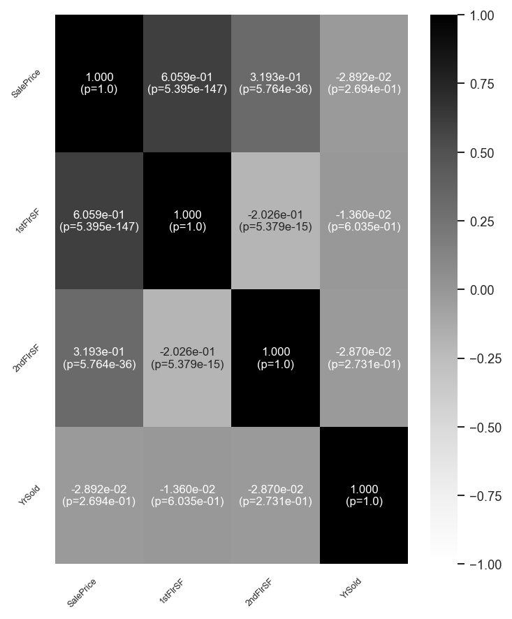
Here’s the same thing as a figure.
[17]:
analyzer.eda().plot_correlation_heatmap(
    ["SalePrice", "1stFlrSF", "2ndFlrSF", "YrSold"], htest=True, figsize=(5, 6)
)
[17]:
Correlations can be compared between a set of numeric variables and a specific numeric variable of interest. Here, we are interested in how square footage and year sold correlate with sale price.
[18]:
analyzer.eda().tabulate_correlation_comparison(
    numeric_vars=["1stFlrSF", "2ndFlrSF", "YrSold"],
    target="SalePrice",
    bonferroni_correction=True,
)
[18]:
| Corr. w SalePrice | p-value (Bonferroni corrected) | |
|---|---|---|
| 1stFlrSF | 0.606 | 1.618e-146 |
| 2ndFlrSF | 0.319 | 1.729e-35 |
| YrSold | -0.029 | 8.082e-01 |
We leverage the Python tableone package to make descriptive exploratory tables.
[19]:
analyzer.eda().tabulate_tableone(
    vars=["SalePrice", "1stFlrSF", "2ndFlrSF", "YrSold", "BldgType"],
    stratify_by="GarageFinish",
)
[19]:
| Grouped by GarageFinish | ||||||||
|---|---|---|---|---|---|---|---|---|
| Missing | Overall | Fin | RFn | Unf | P-Value | Test | ||
| n | 1460 | 352 | 422 | 605 | ||||
| SalePrice, mean (SD) | 0 | 180921.2 (79442.5) | 240052.7 (96960.6) | 202068.9 (63536.2) | 142156.4 (46498.5) | <0.001 | One-way ANOVA | |
| 1stFlrSF, mean (SD) | 0 | 1162.6 (386.6) | 1326.5 (479.3) | 1240.6 (351.5) | 1046.0 (298.4) | <0.001 | One-way ANOVA | |
| 2ndFlrSF, mean (SD) | 0 | 347.0 (436.5) | 452.3 (503.3) | 341.1 (448.2) | 304.5 (381.3) | <0.001 | One-way ANOVA | |
| YrSold, n (%) | 2006 | 314 (21.5) | 74 (21.0) | 92 (21.8) | 133 (22.0) | 0.997 | Chi-squared | |
| 2007 | 329 (22.5) | 79 (22.4) | 93 (22.0) | 140 (23.1) | ||||
| 2008 | 304 (20.8) | 74 (21.0) | 89 (21.1) | 118 (19.5) | ||||
| 2009 | 338 (23.2) | 85 (24.1) | 95 (22.5) | 143 (23.6) | ||||
| 2010 | 175 (12.0) | 40 (11.4) | 53 (12.6) | 71 (11.7) | ||||
| BldgType, n (%) | 1Fam | 1220 (83.6) | 296 (84.1) | 365 (86.5) | 505 (83.5) | <0.001 | Chi-squared | |
| 2fmCon | 31 (2.1) | 3 (0.9) | 2 (0.5) | 17 (2.8) | ||||
| Duplex | 52 (3.6) | 2 (0.6) | 1 (0.2) | 37 (6.1) | ||||
| Twnhs | 43 (2.9) | 2 (0.6) | 8 (1.9) | 28 (4.6) | ||||
| TwnhsE | 114 (7.8) | 49 (13.9) | 46 (10.9) | 18 (3.0) | ||||
Section 3: Regression Analysis
TableMage accelerates regression analyses. Let’s start with a basic example on the house prices dataset.
[20]:
data_path = curr_dir.parent / "demo" / "regression" / "house_price_data" / "data.csv"
df = pd.read_csv(data_path, index_col=0)
analyzer = tm.Analyzer(
    df, test_size=0.2, split_seed=42, verbose=True, name="House Prices"
)
analyzer
UPDT: Analyzer initialized for dataset 'House Prices'.
[20]:
========================================================================================
House Prices
----------------------------------------------------------------------------------------
Train shape: (1168, 80)                      Test shape: (292, 80)
----------------------------------------------------------------------------------------
Categorical variables:
  'Alley', 'BldgType', 'BsmtCond', 'BsmtExposure', 'BsmtFinType1', 'BsmtFinType2',
  'BsmtQual', 'CentralAir', 'Condition1', 'Condition2', 'Electrical', 'ExterCond',
  'ExterQual', 'Exterior1st', 'Exterior2nd', 'Fence', 'FireplaceQu', 'Foundation',
  'Functional', 'GarageCond', 'GarageFinish', 'GarageQual', 'GarageType', 'Heating',
  'HeatingQC', 'HouseStyle', 'KitchenQual', 'LandContour', 'LandSlope', 'LotConfig',
  'LotShape', 'MSZoning', 'MasVnrType', 'MiscFeature', 'Neighborhood', 'PavedDrive',
  'PoolQC', 'RoofMatl', 'RoofStyle', 'SaleCondition', 'SaleType', 'Street', 'Utilities'

Numeric variables:
  '1stFlrSF', '2ndFlrSF', '3SsnPorch', 'BedroomAbvGr', 'BsmtFinSF1', 'BsmtFinSF2',
  'BsmtFullBath', 'BsmtHalfBath', 'BsmtUnfSF', 'EnclosedPorch', 'Fireplaces',
  'FullBath', 'GarageArea', 'GarageCars', 'GarageYrBlt', 'GrLivArea', 'HalfBath',
  'KitchenAbvGr', 'LotArea', 'LotFrontage', 'LowQualFinSF', 'MSSubClass', 'MasVnrArea',
  'MiscVal', 'MoSold', 'OpenPorchSF', 'OverallCond', 'OverallQual', 'PoolArea',
  'SalePrice', 'ScreenPorch', 'TotRmsAbvGrd', 'TotalBsmtSF', 'WoodDeckSF', 'YearBuilt',
  'YearRemodAdd', 'YrSold'
========================================================================================
Let’s first preprocess the data some.
[21]:
analyzer.dropna(include_vars=["SalePrice"]).impute(
    include_vars=["1stFlrSF", "2ndFlrSF", "YrSold"]
)
UPDT: Dropped 0 rows with missing values from train and 0 rows from test.
NOTE: Numeric variables '1stFlrSF', '2ndFlrSF', 'YrSold' have no missing values. Imputer
      will consider all specified variables regardless.
UPDT: Imputed missing values with strategy 'median' for numeric variables '1stFlrSF',
      '2ndFlrSF', 'YrSold'.
[21]:
========================================================================================
House Prices
----------------------------------------------------------------------------------------
Train shape: (1168, 80)                      Test shape: (292, 80)
----------------------------------------------------------------------------------------
Categorical variables:
  'Alley', 'BldgType', 'BsmtCond', 'BsmtExposure', 'BsmtFinType1', 'BsmtFinType2',
  'BsmtQual', 'CentralAir', 'Condition1', 'Condition2', 'Electrical', 'ExterCond',
  'ExterQual', 'Exterior1st', 'Exterior2nd', 'Fence', 'FireplaceQu', 'Foundation',
  'Functional', 'GarageCond', 'GarageFinish', 'GarageQual', 'GarageType', 'Heating',
  'HeatingQC', 'HouseStyle', 'KitchenQual', 'LandContour', 'LandSlope', 'LotConfig',
  'LotShape', 'MSZoning', 'MasVnrType', 'MiscFeature', 'Neighborhood', 'PavedDrive',
  'PoolQC', 'RoofMatl', 'RoofStyle', 'SaleCondition', 'SaleType', 'Street', 'Utilities'

Numeric variables:
  '1stFlrSF', '2ndFlrSF', '3SsnPorch', 'BedroomAbvGr', 'BsmtFinSF1', 'BsmtFinSF2',
  'BsmtFullBath', 'BsmtHalfBath', 'BsmtUnfSF', 'EnclosedPorch', 'Fireplaces',
  'FullBath', 'GarageArea', 'GarageCars', 'GarageYrBlt', 'GrLivArea', 'HalfBath',
  'KitchenAbvGr', 'LotArea', 'LotFrontage', 'LowQualFinSF', 'MSSubClass', 'MasVnrArea',
  'MiscVal', 'MoSold', 'OpenPorchSF', 'OverallCond', 'OverallQual', 'PoolArea',
  'SalePrice', 'ScreenPorch', 'TotRmsAbvGrd', 'TotalBsmtSF', 'WoodDeckSF', 'YearBuilt',
  'YearRemodAdd', 'YrSold'
========================================================================================
It’s really easy to fit an OLS model.
[22]:
report = analyzer.ols(target="SalePrice", predictors=["1stFlrSF", "2ndFlrSF", "YrSold"])
report
[22]:
========================================================================================
Ordinary Least Squares Regression Report
----------------------------------------------------------------------------------------
Target variable:
  'SalePrice'

Predictor variables (3):
  '1stFlrSF', '2ndFlrSF', 'YrSold'
----------------------------------------------------------------------------------------
Metrics:
  Train (1168)                               Test (292)
    R2:       0.548                            R2:       0.636
    Adj. R2:  0.547                            Adj. R2:  0.633
    RMSE:     51925.911                        RMSE:     52810.739
----------------------------------------------------------------------------------------
Coefficients:
                            Estimate         Std. Error            p-value
  Predictor
  const                  -876198.651        2181846.129              0.688
  1stFlrSF                   137.096             15.182              0.000
  2ndFlrSF                    80.969              6.990              0.000
  YrSold                     432.707           1086.173              0.690
========================================================================================
[23]:
report.metrics(dataset="both")
[23]:
| OLS Linear Model | ||
|---|---|---|
| Dataset | Statistic | |
| train | rmse | 51925.911 |
| mae | 34482.403 | |
| mape | 0.205 | |
| pearsonr | 0.740 | |
| spearmanr | 0.771 | |
| r2 | 0.548 | |
| adjr2 | 0.547 | |
| n_obs | 1168.000 | |
| test | rmse | 52810.739 |
| mae | 35310.444 | |
| mape | 0.212 | |
| pearsonr | 0.813 | |
| spearmanr | 0.806 | |
| r2 | 0.636 | |
| adjr2 | 0.633 | |
| n_obs | 292.000 |
[24]:
report.coefs(format="coef(se)|pval")
[24]:
| Estimate (Std. Error) | p-value | |
|---|---|---|
| const | -876198.651 (2181846.129) | 0.688 |
| 1stFlrSF | 137.096 (15.182) | 0.000 |
| 2ndFlrSF | 80.969 (6.99) | 0.000 |
| YrSold | 432.707 (1086.173) | 0.690 |
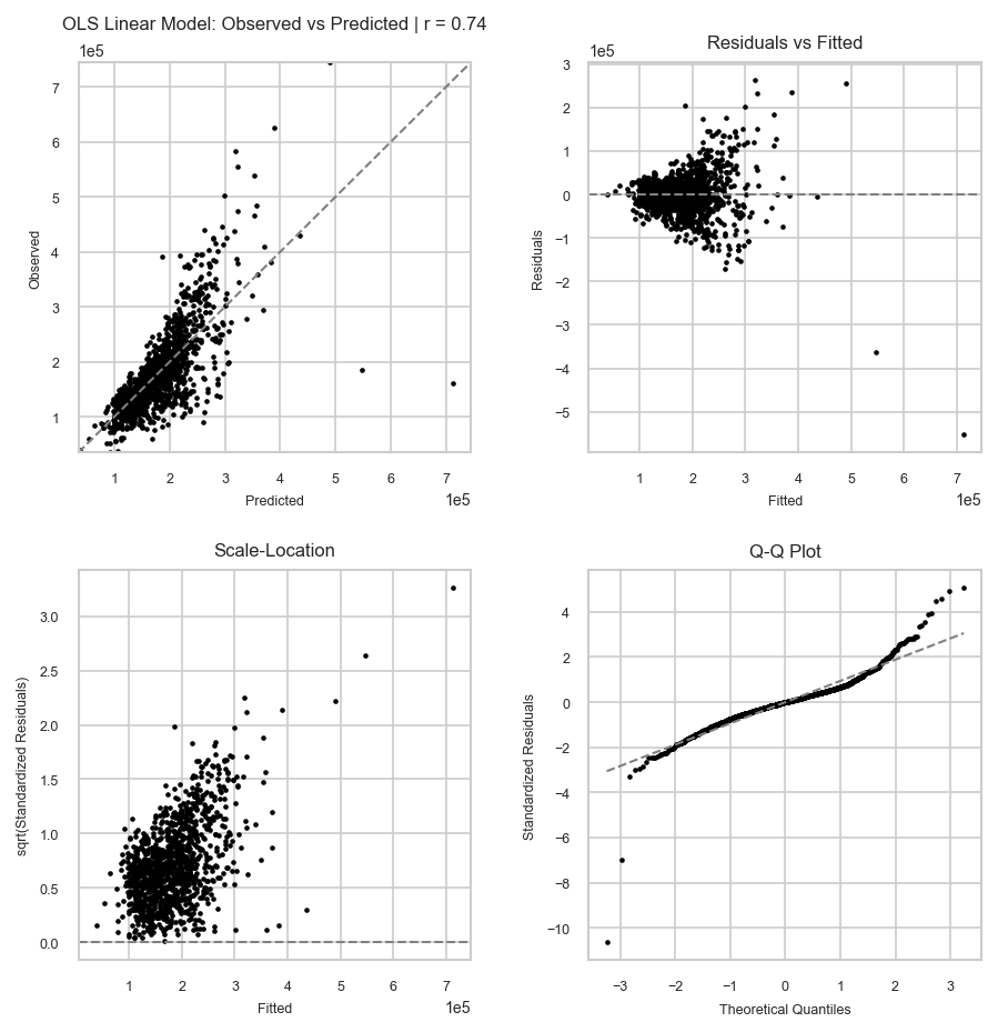
[25]:
report.plot_diagnostics("train")
[25]:
Section 4: Causal Inference
In this section, we use the TableMage package to estimate the causal effect of education on wage using a labor market dataset.
First, we load the datsaset, as shown below.
[26]:
data_path = curr_dir.parent / "demo" / "causal" / "data" / "card.csv"
df_causal = pd.read_csv(data_path, index_col=0)
Next, we initialize an Analyzer.
[27]:
analyzer = tm.Analyzer(
    df_causal, test_size=0.2, split_seed=42, verbose=True, name="Labor Market Behavior"
)
analyzer
UPDT: Analyzer initialized for dataset 'Labor Market Behavior'.
[27]:
========================================================================================
Labor Market Behavior
----------------------------------------------------------------------------------------
Train shape: (2408, 34)                      Test shape: (602, 34)
----------------------------------------------------------------------------------------
Categorical variables:
  None

Numeric variables:
  'IQ', 'KWW', 'age', 'black', 'educ', 'educ_binary', 'enroll', 'exper', 'expersq',
  'fatheduc', 'libcrd14', 'lwage', 'married', 'momdad14', 'motheduc', 'nearc2',
  'nearc4', 'reg661', 'reg662', 'reg663', 'reg664', 'reg665', 'reg666', 'reg667',
  'reg668', 'reg669', 'sinmom14', 'smsa', 'smsa66', 'south', 'south66', 'step14',
  'wage', 'weight'
========================================================================================
We can now make a basic causal inference model.
[28]:
causal_model = analyzer.causal(
    treatment="educ_binary",
    outcome="lwage",
    confounders=[
        "exper",
        "expersq",
        "black",
        "smsa",
        "south",
        "smsa66",
        "reg662",
        "reg663",
        "reg664",
        "reg665",
        "reg666",
        "reg667",
        "reg668",
        "reg669",
    ],
)
We can compute the difference in means naively.
[29]:
report = causal_model.estimate_ate(method="naive")
report
[29]:
========================================================================================
Causal Effect Estimation Report
----------------------------------------------------------------------------------------
Estimate: 0.194                             Std Err: 0.016
Estimand: Avg Trmt Effect (ATE)             p-value: 0.000e+00
----------------------------------------------------------------------------------------
Treatment variable:
  'educ_binary'

Outcome variable:
  'lwage'

Confounders:
  'exper', 'expersq', 'black', 'smsa', 'south', 'smsa66', 'reg662', 'reg663', 'reg664',
  'reg665', 'reg666', 'reg667', 'reg668', 'reg669'
----------------------------------------------------------------------------------------
Method:
  Naive Estimator (Difference in Means)
========================================================================================
With the introduction of these cofounders, we should estimate the ATE with a method that takes confounding into account. Let’s use outcome regression.
[30]:
report = causal_model.estimate_ate(method="outcome_regression", robust_se="nonrobust")
report
[30]:
========================================================================================
Causal Effect Estimation Report
----------------------------------------------------------------------------------------
Estimate: 0.238                             Std Err: 0.017
Estimand: Avg Trmt Effect (ATE)             p-value: 5.107e-42
----------------------------------------------------------------------------------------
Treatment variable:
  'educ_binary'

Outcome variable:
  'lwage'

Confounders:
  'exper', 'expersq', 'black', 'smsa', 'south', 'smsa66', 'reg662', 'reg663', 'reg664',
  'reg665', 'reg666', 'reg667', 'reg668', 'reg669'
----------------------------------------------------------------------------------------
Method:
  Outcome Regression
========================================================================================
Here’s another example where we apply the IPW (inverse probability weighting) estimator to estimate the ATT (average treatment effect on the treated).
[31]:
report = causal_model.estimate_att(method="ipw_weighted_regression", robust_se="HC0")
report
[31]:
========================================================================================
Causal Effect Estimation Report
----------------------------------------------------------------------------------------
Estimate: 0.232                             Std Err: 0.020
Estimand: Avg Trmt Effect on Trtd (ATT)     p-value: 1.975e-31
----------------------------------------------------------------------------------------
Treatment variable:
  'educ_binary'

Outcome variable:
  'lwage'

Confounders:
  'exper', 'expersq', 'black', 'smsa', 'south', 'smsa66', 'reg662', 'reg663', 'reg664',
  'reg665', 'reg666', 'reg667', 'reg668', 'reg669'
----------------------------------------------------------------------------------------
Method:
  Inverse Probability Weighting (IPW) Weighted Regression
========================================================================================
Section 5: Machine Learning
Now, let’s work through how to do machine learning model benchmarking using TableMage.
To begin, let’s use the house price data once again.
[32]:
import joblib
import numpy as np

data_path = curr_dir.parent / "demo" / "regression" / "house_price_data" / "data.csv"
df = pd.read_csv(data_path, index_col=0)
analyzer = tm.Analyzer(
    df, test_size=0.2, split_seed=42, verbose=True, name="House Prices"
)
analyzer
UPDT: Analyzer initialized for dataset 'House Prices'.
[32]:
========================================================================================
House Prices
----------------------------------------------------------------------------------------
Train shape: (1168, 80)                      Test shape: (292, 80)
----------------------------------------------------------------------------------------
Categorical variables:
  'Alley', 'BldgType', 'BsmtCond', 'BsmtExposure', 'BsmtFinType1', 'BsmtFinType2',
  'BsmtQual', 'CentralAir', 'Condition1', 'Condition2', 'Electrical', 'ExterCond',
  'ExterQual', 'Exterior1st', 'Exterior2nd', 'Fence', 'FireplaceQu', 'Foundation',
  'Functional', 'GarageCond', 'GarageFinish', 'GarageQual', 'GarageType', 'Heating',
  'HeatingQC', 'HouseStyle', 'KitchenQual', 'LandContour', 'LandSlope', 'LotConfig',
  'LotShape', 'MSZoning', 'MasVnrType', 'MiscFeature', 'Neighborhood', 'PavedDrive',
  'PoolQC', 'RoofMatl', 'RoofStyle', 'SaleCondition', 'SaleType', 'Street', 'Utilities'

Numeric variables:
  '1stFlrSF', '2ndFlrSF', '3SsnPorch', 'BedroomAbvGr', 'BsmtFinSF1', 'BsmtFinSF2',
  'BsmtFullBath', 'BsmtHalfBath', 'BsmtUnfSF', 'EnclosedPorch', 'Fireplaces',
  'FullBath', 'GarageArea', 'GarageCars', 'GarageYrBlt', 'GrLivArea', 'HalfBath',
  'KitchenAbvGr', 'LotArea', 'LotFrontage', 'LowQualFinSF', 'MSSubClass', 'MasVnrArea',
  'MiscVal', 'MoSold', 'OpenPorchSF', 'OverallCond', 'OverallQual', 'PoolArea',
  'SalePrice', 'ScreenPorch', 'TotRmsAbvGrd', 'TotalBsmtSF', 'WoodDeckSF', 'YearBuilt',
  'YearRemodAdd', 'YrSold'
========================================================================================
Feel free to perform any preprocessing steps.
[33]:
analyzer.dropna(
    include_vars=["SalePrice"]
).drop_highly_missing_vars(  # drop variables with more than 30% missing values
    exclude_vars=["SalePrice"], threshold=0.3
).impute(  # impute missing values
    exclude_vars=["SalePrice"],
    numeric_strategy="5nn",
    categorical_strategy="most_frequent",
).scale(  # scale numeric variables
    exclude_vars=["SalePrice"], strategy="standardize"
)
UPDT: Dropped 0 rows with missing values from train and 0 rows from test.
UPDT: Dropped variables 'Alley', 'Fence', 'FireplaceQu', 'MasVnrType', 'MiscFeature',
      'PoolQC' with at least 30.0% of values missing.
NOTE: Numeric variables 'ScreenPorch', 'GrLivArea', 'GarageCars', '2ndFlrSF',
      'BsmtFinSF2', 'PoolArea', 'BsmtFullBath', 'YearRemodAdd', 'WoodDeckSF',
      'BsmtUnfSF', 'TotalBsmtSF', 'MiscVal', 'BsmtHalfBath', 'OverallCond',
      'BedroomAbvGr', 'BsmtFinSF1', 'MoSold', 'OpenPorchSF', 'TotRmsAbvGrd', 'FullBath',
      'YearBuilt', 'GarageArea', '3SsnPorch', 'OverallQual', '1stFlrSF', 'YrSold',
      'LowQualFinSF', 'Fireplaces', 'HalfBath', 'MSSubClass', 'KitchenAbvGr', 'LotArea',
      'EnclosedPorch' have no missing values. Imputer will consider all specified
      variables regardless.
NOTE: Categorical variables 'RoofMatl', 'LotConfig', 'LandContour', 'Foundation',
      'Exterior1st', 'HeatingQC', 'Condition1', 'Neighborhood', 'RoofStyle', 'Street',
      'SaleCondition', 'Condition2', 'HouseStyle', 'Functional', 'ExterQual',
      'LandSlope', 'SaleType', 'LotShape', 'BldgType', 'Heating', 'ExterCond',
      'Exterior2nd', 'PavedDrive', 'Utilities', 'CentralAir', 'KitchenQual', 'MSZoning'
      have no missing values. Imputer will consider all specified variables regardless.
UPDT: Imputed missing values with strategy '5nn' for numeric variables '1stFlrSF',
      '2ndFlrSF', '3SsnPorch', 'BedroomAbvGr', 'BsmtFinSF1', 'BsmtFinSF2',
      'BsmtFullBath', 'BsmtHalfBath', 'BsmtUnfSF', 'EnclosedPorch', 'Fireplaces',
      'FullBath', 'GarageArea', 'GarageCars', 'GarageYrBlt', 'GrLivArea', 'HalfBath',
      'KitchenAbvGr', 'LotArea', 'LotFrontage', 'LowQualFinSF', 'MSSubClass',
      'MasVnrArea', 'MiscVal', 'MoSold', 'OpenPorchSF', 'OverallCond', 'OverallQual',
      'PoolArea', 'ScreenPorch', 'TotRmsAbvGrd', 'TotalBsmtSF', 'WoodDeckSF',
      'YearBuilt', 'YearRemodAdd', 'YrSold' and strategy 'most_frequent' for categorical
      variables 'BldgType', 'BsmtCond', 'BsmtExposure', 'BsmtFinType1', 'BsmtFinType2',
      'BsmtQual', 'CentralAir', 'Condition1', 'Condition2', 'Electrical', 'ExterCond',
      'ExterQual', 'Exterior1st', 'Exterior2nd', 'Foundation', 'Functional',
      'GarageCond', 'GarageFinish', 'GarageQual', 'GarageType', 'Heating', 'HeatingQC',
      'HouseStyle', 'KitchenQual', 'LandContour', 'LandSlope', 'LotConfig', 'LotShape',
      'MSZoning', 'Neighborhood', 'PavedDrive', 'RoofMatl', 'RoofStyle',
      'SaleCondition', 'SaleType', 'Street', 'Utilities'.
UPDT: Scaled variables 'GarageYrBlt', 'ScreenPorch', 'LotFrontage', 'GrLivArea',
      'GarageCars', '2ndFlrSF', 'BsmtFinSF2', 'PoolArea', 'BsmtFullBath',
      'YearRemodAdd', 'WoodDeckSF', 'BsmtUnfSF', 'TotalBsmtSF', 'MiscVal',
      'BsmtHalfBath', 'OverallCond', 'BedroomAbvGr', 'MasVnrArea', 'BsmtFinSF1',
      'MoSold', 'OpenPorchSF', 'TotRmsAbvGrd', 'FullBath', 'YearBuilt', 'GarageArea',
      '3SsnPorch', 'OverallQual', '1stFlrSF', 'YrSold', 'LowQualFinSF', 'Fireplaces',
      'HalfBath', 'MSSubClass', 'KitchenAbvGr', 'LotArea', 'EnclosedPorch' using
      strategy 'standardize'.
[33]:
========================================================================================
House Prices
----------------------------------------------------------------------------------------
Train shape: (1168, 74)                      Test shape: (292, 74)
----------------------------------------------------------------------------------------
Categorical variables:
  'BldgType', 'BsmtCond', 'BsmtExposure', 'BsmtFinType1', 'BsmtFinType2', 'BsmtQual',
  'CentralAir', 'Condition1', 'Condition2', 'Electrical', 'ExterCond', 'ExterQual',
  'Exterior1st', 'Exterior2nd', 'Foundation', 'Functional', 'GarageCond',
  'GarageFinish', 'GarageQual', 'GarageType', 'Heating', 'HeatingQC', 'HouseStyle',
  'KitchenQual', 'LandContour', 'LandSlope', 'LotConfig', 'LotShape', 'MSZoning',
  'Neighborhood', 'PavedDrive', 'RoofMatl', 'RoofStyle', 'SaleCondition', 'SaleType',
  'Street', 'Utilities'

Numeric variables:
  '1stFlrSF', '2ndFlrSF', '3SsnPorch', 'BedroomAbvGr', 'BsmtFinSF1', 'BsmtFinSF2',
  'BsmtFullBath', 'BsmtHalfBath', 'BsmtUnfSF', 'EnclosedPorch', 'Fireplaces',
  'FullBath', 'GarageArea', 'GarageCars', 'GarageYrBlt', 'GrLivArea', 'HalfBath',
  'KitchenAbvGr', 'LotArea', 'LotFrontage', 'LowQualFinSF', 'MSSubClass', 'MasVnrArea',
  'MiscVal', 'MoSold', 'OpenPorchSF', 'OverallCond', 'OverallQual', 'PoolArea',
  'SalePrice', 'ScreenPorch', 'TotRmsAbvGrd', 'TotalBsmtSF', 'WoodDeckSF', 'YearBuilt',
  'YearRemodAdd', 'YrSold'
========================================================================================
We can use the regress function in our analyzer to properly benchmark certain models. In this case, we compare the Random Forest, XGBoost, and linear regression models.
[34]:
reg_report = analyzer.regress(
    models=[
        tm.ml.LinearR("l2"),
        tm.ml.TreesR("random_forest"),
        tm.ml.TreesR("xgboost"),
    ],
    target="SalePrice",
    predictors=["1stFlrSF", "2ndFlrSF", "YrSold", "BldgType", "MSZoning", "LotShape"],
    feature_selectors=[tm.fs.BorutaFSR()],  # select features
)
PROG: Fitting 'BorutaFSR'.
UPDT: Fitting model 'LinearR(l2)'.
PROG: Fitting 'LinearR(l2)'. Search method: OptunaSearchCV (100 trials, 500 total fits).

UPDT: Successfully evaluated model 'LinearR(l2)'.
UPDT: Fitting model 'TreesR(random_forest)'.
PROG: Fitting 'TreesR(random_forest)'. Search method: OptunaSearchCV (100 trials, 500
      total fits).
UPDT: Successfully evaluated model 'TreesR(random_forest)'.
UPDT: Fitting model 'TreesR(xgboost)'.
PROG: Fitting 'TreesR(xgboost)'. Search method: OptunaSearchCV (100 trials, 500 total
      fits).
UPDT: Successfully evaluated model 'TreesR(xgboost)'.
Lastly, we can compare model metrics and save models for future use.
[35]:
# Compare model performance
display(reg_report.metrics("test"))

# Predict on new data
new_df = df.sample(frac=0.3)
new_df = new_df.drop(columns=["SalePrice"])

y_pred = reg_report.model("LinearR(l2)").sklearn_pipeline().predict(new_df)

# Save model as sklearn pipeline
joblib.dump(reg_report.model("LinearR(l2)").sklearn_pipeline(), "l2_pipeline.joblib")

# Load model and predict on new data
y_pred_from_save = joblib.load("l2_pipeline.joblib").predict(new_df)
assert np.allclose(y_pred, y_pred_from_save)
| LinearR(l2) | TreesR(random_forest) | TreesR(xgboost) | |
|---|---|---|---|
| Statistic | |||
| rmse | 50294.432 | 47174.405 | 45710.156 |
| mae | 32321.420 | 30499.842 | 29765.441 |
| mape | 0.194 | 0.187 | 0.180 |
| pearsonr | 0.832 | 0.849 | 0.859 |
| spearmanr | 0.861 | 0.866 | 0.870 |
| r2 | 0.670 | 0.710 | 0.728 |
| adjr2 | 0.666 | 0.706 | 0.724 |
| n_obs | 292.000 | 292.000 | 292.000 |
Section 6: Conversational Data Analysis
In this section, we demonstrate how to use TableMage’s conversational data analysis capabilities. This is particularly useful for no-code use of the package, helping those that may not have the background necessary to do thorough data analysis on their datasets.
First, we enable the use of agents in TableMage with the tm.use_agents() function.
[36]:
import tablemage as tm

data_path = curr_dir.parent / "demo" / "regression" / "house_price_data" / "data.csv"
df = pd.read_csv(data_path, index_col=0)
[37]:
from IPython.display import Markdown

tm.use_agents()
None of PyTorch, TensorFlow >= 2.0, or Flax have been found. Models won't be available and only tokenizers, configuration and file/data utilities can be used.
UPDT: The 'tablemage.agents' module has been imported.
We then set the API key for the OpenAI agent using the tm.agents.set_key method. We also configure the agent to use the GPT-5.1 model with the tm.agents.options.set_llm method.
[38]:
tm.agents.set_key(
    llm_type="openai",
    api_key="your-key-here",
)
tm.agents.options.set_llm(llm_type="openai", model_name="gpt-5.1")
We initialize a ChatDA agent with the training dataset df and a test size of 20%.
[39]:
agent = tm.agents.ChatDA(df=df, test_size=0.2, verbose=False)
We interact with the agent through the chat method.
[40]:
response = agent.chat("Tell me about the dataset.")
Markdown(response)
[40]:
Here’s what your summary tells us about the dataset:
Size and structure
Training set: 1,168 rows × 80 columns
Test set: 292 rows × 80 columns
This is a moderate-sized tabular dataset, typical for housing/real estate problems.
Variable types
37 numeric variables – continuous or discrete counts, e.g.:
Size-related:
1stFlrSF,2ndFlrSF,GrLivArea,TotalBsmtSF,GarageArea,LotArea,MasVnrArea,WoodDeckSF,OpenPorchSF,EnclosedPorch,ScreenPorch,PoolArea,LowQualFinSF,3SsnPorchCounts:
BedroomAbvGr,TotRmsAbvGrd,FullBath,HalfBath,BsmtFullBath,BsmtHalfBath,Fireplaces,GarageCars,KitchenAbvGrQuality/overall scores (ordinal, but stored numeric):
OverallQual,OverallCondTime-related:
YearBuilt,YearRemodAdd,GarageYrBlt,YrSold,MoSoldOthers:
MSSubClass,LotFrontage,MiscVal, and crucially ``SalePrice``.
43 categorical variables – building, quality, location, and condition descriptors, e.g.:
Location/land:
Neighborhood,MSZoning,LotShape,LandContour,LotConfig,LandSlope,Street,AlleyExterior:
Exterior1st,Exterior2nd,RoofStyle,RoofMatlBasement / garage:
BsmtQual,BsmtCond,BsmtExposure,BsmtFinType1,BsmtFinType2,GarageType,GarageFinish,GarageQual,GarageCondQuality/condition (ordinal but stored as categories):
ExterQual,ExterCond,HeatingQC,KitchenQual,Functional,FireplaceQu,Fence,PoolQCHouse configuration:
BldgType,HouseStyle,Foundation,Heating,CentralAir,PavedDriveTransaction:
SaleType,SaleCondition,Utilities,MiscFeature
Likely task
Presence of ``SalePrice`` (numeric) suggests a supervised regression problem: predicting house sale prices from structural, quality, and location features.
The test set with the same 80 features (presumably without
SalePrice) is likely intended for out-of-sample evaluation or competition-style scoring.
Characteristics/considerations
Many variables are housing attributes (structure + location + condition), matching the classic Ames housing dataset style.
You have a mix of:
Continuous features (areas, frontage, lot size),
Discrete counts (rooms, baths, cars),
Ordinal categories coded as text (e.g., quality from Poor→Excellent),
Potentially sparse features (e.g.,
PoolQC,MiscFeature,Alleyoften have many missing values in similar datasets).
There are many categorical variables (43), so modeling will require:
Some form of encoding (e.g., one-hot encoding),
Care about high-cardinality variables such as
Neighborhood.
If you’d like, the next steps I’d suggest are:
Show summary stats of ``SalePrice`` (distribution, range, skewness).
Inspect missing values by variable.
Look at simple relationships with price (e.g.,
OverallQual,GrLivArea,Neighborhood).
[41]:
response = agent.chat("""Provide the summary statistics.
    Also help me figure out which variables are highly correlated with SalePrice.
    """)
Markdown(response)
[41]:
Here’s what we can say from your data.
1. Summary statistics
1.1. Target variable: SalePrice
Count: 1,460
Mean: 180,921
Std dev: 79,443
Min: 34,900
25%: 129,975
Median (50%): 163,000
75%: 214,000
Max: 755,000
Implications:
Prices are quite spread out (std ~ 80k).
Strong right skew (few very expensive houses).
1.2. Numeric variables (high level)
For each numeric variable you have:
min,max,mean,std,varianceQuartiles (q1, median, q3)
Shape:
skew,kurtosisMissingness:
n_missing,missing_rate
Examples:
GrLivArea(above-ground living area):Mean: 1,515 sq ft, Std: 525, Min: 334, Max: 5,642
Skew ~ 1.37 (right-skewed, some very large houses)
No missing values
OverallQual(overall material/finish quality, 1–10):Mean: 6.10, Std: 1.38, IQR: 5–7
Variables with notable missingness:
LotFrontage: 17.7% missingGarageYrBlt: 5.5% missingMasVnrArea: 0.5% missing
(If you want, I can list the full numeric summary table explicitly, but it’s quite long.)
1.3. Categorical variables (high level)
For each categorical variable you have:
Number of unique categories
Most common and least common category
Missingness
Notable:
Very high missingness:
PoolQC: 99.5% missingMiscFeature: 96.3% missingAlley: 93.8% missingFence: 80.8% missingMasVnrType: 59.7% missingFireplaceQu: 47.3% missing
Neighborhood has 25 categories; most common is
NAmes.
These highly-missing variables may need special treatment (e.g., treat “missing” as its own category, or drop if not informative).
3. Suggested next steps
If you’d like to go further, we can:
Visualize
SalePricevs. these top predictors (scatterplots, log-transform if needed).Check correlations among predictors (to understand multicollinearity).
Start a simple baseline model using just the top few variables.
[42]:
response = agent.chat("""Help me predict the SalePrice with linear regression.
    Choose the predictors you think are most relevant.
    """)
Markdown(response)
[42]:
Here’s a linear regression model for SalePrice using a focused set of strong, interpretable predictors.
1. Predictors I chose
Based on prior correlation analysis and standard practice for this dataset, I used these numeric predictors:
OverallQual– overall material/finish qualityGrLivArea– above-ground living area (sq ft)GarageCars– number of car spaces in garageGarageArea– size of garage (sq ft)TotalBsmtSF– total basement area (sq ft)1stFlrSF– first floor area (sq ft)FullBath– number of full bathrooms above groundTotRmsAbvGrd– total rooms above groundYearBuilt– original construction yearYearRemodAdd– remodel year
All observations were complete for these variables (n = 1,460).
The model is an ordinary least squares (OLS) linear regression:
[ \text{SalePrice} = \beta_0 + \sum `:nbsphinx-math:beta`_j X_j + \varepsilon ]
2. Model performance
R² = 0.774
Adjusted R² = 0.772
Interpretation: about 77% of the variation in SalePrice is explained by this set of predictors.
3. Key coefficients (effects)
Each coefficient is the average change in SalePrice when that predictor increases by 1 unit, holding the others fixed.
Significant predictors (p < 0.05):
OverallQual: +19,605 per 1-point increase (on 1–10 scale)GrLivArea: +51 per additional sq ftGarageCars: +10,418 per additional car spaceTotalBsmtSF: +19.9 per additional sq ft1stFlrSF: +14.2 per additional sq ftFullBath: −6,791 per additional full bath (see note below)YearBuilt: +268 per yearYearRemodAdd: +296 per year
Not statistically significant (in presence of the others):
GarageArea(p ≈ 0.15)TotRmsAbvGrd(p ≈ 0.98)
Notes:
FullBathshowing a negative coefficient is likely due to multicollinearity withGrLivArea,TotRmsAbvGrd, etc. Larger houses tend to have more bathrooms; once you hold the other size variables constant, “extra baths” may not add much or can flip sign.The very large condition number (~4.7e5) further indicates multicollinearity among size-related variables.
The intercept:
const≈ −1,186,194 This isn’t directly meaningful because it corresponds to an impossible combination of predictor values (e.g., year 0, zero area, etc.), so we typically ignore its standalone interpretation.
4. How to use this model
In plain form, your prediction equation is approximately:
[
]
(Values in currency units are in the same units as SalePrice in your data.)
5. Suggested refinements
If you want to improve or simplify this model, next steps could be:
Drop weak predictors (
GarageArea,TotRmsAbvGrd) and refit.Reduce multicollinearity by:
Choosing one or two core size measures (e.g.,
GrLivArea,TotalBsmtSF) instead of several overlapping ones, orCreating composite features (e.g., total finished area).
Consider a log-transform of
SalePrice(and maybe heavily-skewed predictors) to better handle skew and outliers.
If you’d like, I can:
Refit a simplified model with fewer, more stable predictors, or
Train a model on
log(SalePrice)and show you the updated performance and coefficients.
[43]:
response = agent.chat(
    """Fit some machine learning models to try to obtain better predictive performance.
    Do whatever you think would be best for performance.
    Let me know which model is best and how it performs.
    Tell me also how you trained that model.
    """
)
Markdown(response)
[43]:
Here’s what I did and what worked best.
1. Models trained and comparison
I focused on predicting SalePrice using a strong numeric subset:
Predictors used (selected via Boruta feature selection):
OverallQualGrLivAreaGarageCarsGarageAreaTotalBsmtSF1stFlrSFFullBathYearBuiltYearRemodAdd
Then I trained and tuned these regression models, with an internal train/test split (about 80/20: 1,168 train, 292 test):
Linear models: OLS, Ridge, Lasso, ElasticNet
Nonlinear: Random Forest (RF), XGBoost
SVM (RBF kernel)
Test-set performance (the metric that really matters):
OLS: R² = 0.797, RMSE ≈ 39,459
Ridge: R² = 0.797, RMSE ≈ 39,447
Lasso: R² = 0.797, RMSE ≈ 39,459
ElasticNet: R² = 0.797, RMSE ≈ 39,444
Random Forest: R² = 0.876, RMSE ≈ 30,864
XGBoost: R² = 0.866, RMSE ≈ 32,087
SVM: R² ≈ −0.038, RMSE ≈ 89,244 (performed very poorly)
Roughly, Random Forest reduces test RMSE by about:
21–22% vs your OLS baseline (≈ 39.5k → ≈ 30.9k)
2. How the best model (Random Forest) was trained
Data & features
Target:
SalePrice(untransformed).Features:
OverallQual, GrLivArea, GarageCars, GarageArea, TotalBsmtSF, 1stFlrSF, FullBath, YearBuilt, YearRemodAddOnly complete cases were used (no missingness for these variables in this dataset).
Train/test split
Train size: 1,168 observations
Test size: 292 observations
The metrics above are evaluated on this unseen test set.
Model type
Ensemble of decision trees: Random Forest Regressor.
Hyperparameter tuning
I did automated hyperparameter search with cross-validation:
Search space included:
n_estimators: {50, 100, 200, 400}max_depth: integers from 3 to 15 (step 2)min_samples_split: {2, 5, 10}min_samples_leaf: {1, 2, 4}max_features: {‘sqrt’, ‘log2’}
5-fold cross-validation inside the training set.
100 optimization trials to find hyperparameters that best minimized cross-validated error.
Best-found hyperparameters
The final (best) Random Forest used:
n_estimators: 200max_depth: 13min_samples_split: 10min_samples_leaf: 1max_features: ‘log2’
This configuration balances model complexity and overfitting fairly well (high training R² but also high test R²).
Feature importance (from Random Forest)
Relative importance of each predictor in the best model:
OverallQual: 0.298GrLivArea: 0.192GarageCars: 0.137YearBuilt: 0.090TotalBsmtSF: 0.0821stFlrSF: 0.062GarageArea: 0.071FullBath: 0.035YearRemodAdd: 0.034
Interpretation: OverallQual and GrLivArea are the dominant drivers of predictions, but garage capacity, house age, and basement/first-floor area all contribute meaningfully.
3. Summary
Your original OLS linear regression explained ~77–80% of variance with RMSE around 39–40k.
A tuned Random Forest using 9 numeric predictors now explains ~88% of variance with RMSE ~30.9k on a hold-out test set.
That Random Forest is the best-performing model I trained, and it was selected via cross-validated hyperparameter tuning over an ensemble of 200 depth-limited trees.
If you’d like, I can:
Export the exact model formula/settings you’d need to re-implement it in Python or R, or
Try adding more features (including categorical variables via one-hot encoding) to see if we can squeeze out even better performance.
We hope you enjoy TableMage.