TableMage Demonstration
TableMage is a Python package for low-code/conversational data science. In this notebook, we provide a few examples of how the package can be used.
Notebook Contents
Introduction
Exploratory Data Analysis
Regression Analysis
Causal Inference
Machine Learning
Conversational Data Analysis
Section 1: Introduction
1.1: Installation
Let’s first install the package. On a local machine, you simply need to copy-and-paste the following code into your terminal:
git clone https://github.com/ajy25/TableMage.git
cd TableMage
pip install .
If you want to use the conversational data analysis mode, you should replace the last line with the following line:
pip install '.[agents]'
NOTE: If you are a MacOS user, you’ll need to install libomp. It’s a dependency for using XGBoost, a TableMage dependency.
Okay! Let’s run the cell below. On Google Colab, you’ll be prompted to restart the session—this is normal.
[1]:
using_google_colab = False
[2]:
%%capture
!pip uninstall -y tablemage
!rm -rf TableMage
!git clone https://github.com/ajy25/TableMage.git
%cd TableMage
!pip install '.[agents]'
import tablemage as tm
1.2 The Analyzer Class
Now that TableMage is installed, let’s try importing the package. We’ll use a toy dataset from scikit-learn for now.
[3]:
from sklearn.datasets import load_breast_cancer
import pandas as pd

brca_dataset = load_breast_cancer()
df = pd.DataFrame(data=brca_dataset.data, columns=brca_dataset.feature_names)
df["target"] = brca_dataset.target
df.head()
[3]:
| mean radius | mean texture | mean perimeter | mean area | mean smoothness | mean compactness | mean concavity | mean concave points | mean symmetry | mean fractal dimension | ... | worst texture | worst perimeter | worst area | worst smoothness | worst compactness | worst concavity | worst concave points | worst symmetry | worst fractal dimension | target | |
|---|---|---|---|---|---|---|---|---|---|---|---|---|---|---|---|---|---|---|---|---|---|
| 0 | 17.99 | 10.38 | 122.80 | 1001.0 | 0.11840 | 0.27760 | 0.3001 | 0.14710 | 0.2419 | 0.07871 | ... | 17.33 | 184.60 | 2019.0 | 0.1622 | 0.6656 | 0.7119 | 0.2654 | 0.4601 | 0.11890 | 0 |
| 1 | 20.57 | 17.77 | 132.90 | 1326.0 | 0.08474 | 0.07864 | 0.0869 | 0.07017 | 0.1812 | 0.05667 | ... | 23.41 | 158.80 | 1956.0 | 0.1238 | 0.1866 | 0.2416 | 0.1860 | 0.2750 | 0.08902 | 0 |
| 2 | 19.69 | 21.25 | 130.00 | 1203.0 | 0.10960 | 0.15990 | 0.1974 | 0.12790 | 0.2069 | 0.05999 | ... | 25.53 | 152.50 | 1709.0 | 0.1444 | 0.4245 | 0.4504 | 0.2430 | 0.3613 | 0.08758 | 0 |
| 3 | 11.42 | 20.38 | 77.58 | 386.1 | 0.14250 | 0.28390 | 0.2414 | 0.10520 | 0.2597 | 0.09744 | ... | 26.50 | 98.87 | 567.7 | 0.2098 | 0.8663 | 0.6869 | 0.2575 | 0.6638 | 0.17300 | 0 |
| 4 | 20.29 | 14.34 | 135.10 | 1297.0 | 0.10030 | 0.13280 | 0.1980 | 0.10430 | 0.1809 | 0.05883 | ... | 16.67 | 152.20 | 1575.0 | 0.1374 | 0.2050 | 0.4000 | 0.1625 | 0.2364 | 0.07678 | 0 |
5 rows × 31 columns
The Analyzer is the bridge between the data and the analysis methods. Most likely, you’ll want to do some modeling of some sort, such as linear regression or some type of machine learning regression/classification. As such, the Analyzer splits the data into a train dataset and a withheld test dataset upon initialization.
Be careful! The Analyzer will rename variables to make them easily formula-compatible (i.e., replace spaces and other prohibited characters with underscores). It is recommended that you remove spaces and special characters from variable names before you initialize an Analyzer, just to make sure you have full control over the names. A good rule-of-thumb is to avoid punctuation and spaces, with the exceptions of “_” and “.”, which are totally fine. We’ll let Analyzer handle the renaming for now.
[4]:
analyzer = tm.Analyzer(
    df, test_size=0.2, split_seed=42, verbose=True, name="Breast Cancer"
)

# You can also split the dataset yourself, e.g. ...
# df_train, df_test = sklearn.train_test_split(df, random_state=42)
# analyzer = tm.Analyzer(df_train, df_test=df_test)
TableMage is designed for notebooks. Many objects are display-friendly!
[5]:
analyzer
[5]:
========================================================================================
Breast Cancer
----------------------------------------------------------------------------------------
Train shape: (455, 31)                      Test shape: (114, 31)
----------------------------------------------------------------------------------------
Categorical variables:
  None

Numeric variables:
  'area_error', 'compactness_error', 'concave_points_error', 'concavity_error',
  'fractal_dimension_error', 'mean_area', 'mean_compactness', 'mean_concave_points',
  'mean_concavity', 'mean_fractal_dimension', 'mean_perimeter', 'mean_radius',
  'mean_smoothness', 'mean_symmetry', 'mean_texture', 'perimeter_error', 'radius_error',
  'smoothness_error', 'symmetry_error', 'target', 'texture_error', 'worst_area',
  'worst_compactness', 'worst_concave_points', 'worst_concavity',
  'worst_fractal_dimension', 'worst_perimeter', 'worst_radius', 'worst_smoothness',
  'worst_symmetry', 'worst_texture'
========================================================================================
Before we proceed, let’s discuss why TableMage requires train-test splitting upon initialization. TableMage aims to accelerate data science on tabular data. Often, the end goal is to train a model to predict a target, such as whether or not a patient has breast cancer based on geometrical features, or a patient’s billing amoung given the health insurer and disease type. In these cases, it is incredibly important to think in terms of pipelines, especially when transformations must be made to the data. Transformations—including missing data imputation and feature scaling—must be “fit” on the train data only. Performing data transformations based on the entire dataset is a common mistake, even for experienced data scientists.
TableMage handles all of this for you. You can explore the dataset (looking at the entire dataset or only the train or test dataset—your choice), make transformations such as imputation, feature engineering, and scaling, and immediately train a model to predict a target variable, without needing to worry about all the intermediate details! Hopefully, this will be more clear in section 5, when we discuss machine learning.
If you don’t plan on doing any modeling, simply set test_size to 0.
1.3 Submodules
TableMage has two submodules:
ml: Machine learning models
fs: Feature selection models
Let’s print an object from each. These will be discussed in greater detail in section 5.
[6]:
print(tm.ml.LinearC())
print(tm.fs.BorutaFSR())
LinearC(l2)
BorutaFSR
Section 2: Exploratory Data Analysis
Let’s explore a dataset. We’ll use the Kaggle House Prices dataset as an example since it contains a good amount of categorical and numeric features with varying levels of missingness.
[7]:
from pathlib import Path
import matplotlib.pyplot as plt

plt.rcParams["figure.dpi"] = 150

if using_google_colab:
    curr_dir = Path.cwd()
else:
    curr_dir = Path("__notebook__").resolve().parent

data_path = curr_dir / "demo" / "regression" / "house_price_data" / "data.csv"
df = pd.read_csv(data_path, index_col=0)
analyzer = tm.Analyzer(
    df, test_size=0.2, split_seed=42, verbose=True, name="House Prices"
)
analyzer
[7]:
========================================================================================
House Prices
----------------------------------------------------------------------------------------
Train shape: (1168, 80)                      Test shape: (292, 80)
----------------------------------------------------------------------------------------
Categorical variables:
  'Alley', 'BldgType', 'BsmtCond', 'BsmtExposure', 'BsmtFinType1', 'BsmtFinType2',
  'BsmtQual', 'CentralAir', 'Condition1', 'Condition2', 'Electrical', 'ExterCond',
  'ExterQual', 'Exterior1st', 'Exterior2nd', 'Fence', 'FireplaceQu', 'Foundation',
  'Functional', 'GarageCond', 'GarageFinish', 'GarageQual', 'GarageType', 'Heating',
  'HeatingQC', 'HouseStyle', 'KitchenQual', 'LandContour', 'LandSlope', 'LotConfig',
  'LotShape', 'MSZoning', 'MasVnrType', 'MiscFeature', 'Neighborhood', 'PavedDrive',
  'PoolQC', 'RoofMatl', 'RoofStyle', 'SaleCondition', 'SaleType', 'Street', 'Utilities'

Numeric variables:
  '1stFlrSF', '2ndFlrSF', '3SsnPorch', 'BedroomAbvGr', 'BsmtFinSF1', 'BsmtFinSF2',
  'BsmtFullBath', 'BsmtHalfBath', 'BsmtUnfSF', 'EnclosedPorch', 'Fireplaces',
  'FullBath', 'GarageArea', 'GarageCars', 'GarageYrBlt', 'GrLivArea', 'HalfBath',
  'KitchenAbvGr', 'LotArea', 'LotFrontage', 'LowQualFinSF', 'MSSubClass', 'MasVnrArea',
  'MiscVal', 'MoSold', 'OpenPorchSF', 'OverallCond', 'OverallQual', 'PoolArea',
  'SalePrice', 'ScreenPorch', 'TotRmsAbvGrd', 'TotalBsmtSF', 'WoodDeckSF', 'YearBuilt',
  'YearRemodAdd', 'YrSold'
========================================================================================
2.1 Plots
We can begin our analysis by using TableMage to make plots of the dataset.
[8]:
analyzer.eda().plot("SalePrice")
[8]:
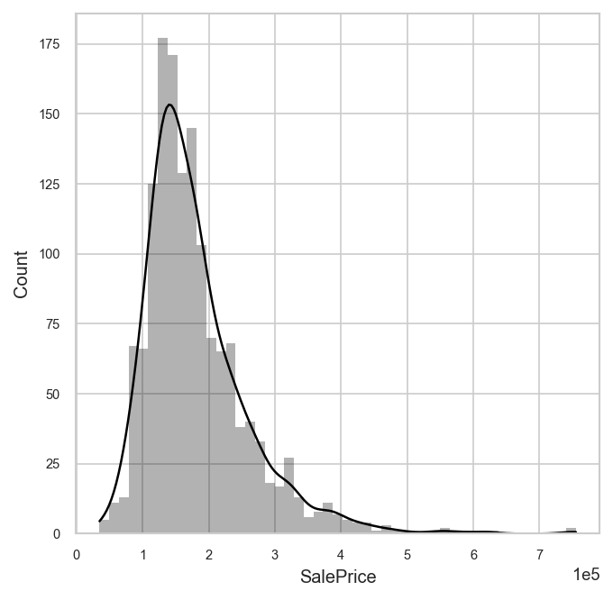
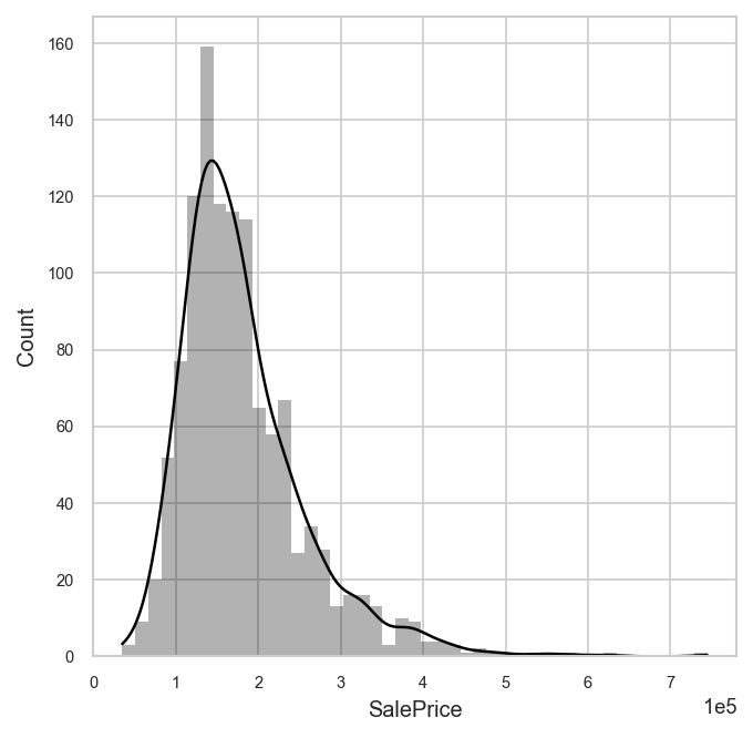
By default, Analyzer considers the entire dataset (train and test) for exploratory analysis. You can change this by specifying which dataset you would like to consider in the analyzer.eda() method.
[9]:
analyzer.eda("train").plot("SalePrice")
[9]:
Let’s plot the sale price versus 1st floor square footage.
[10]:
analyzer.eda().plot("SalePrice", "1stFlrSF")
[10]:
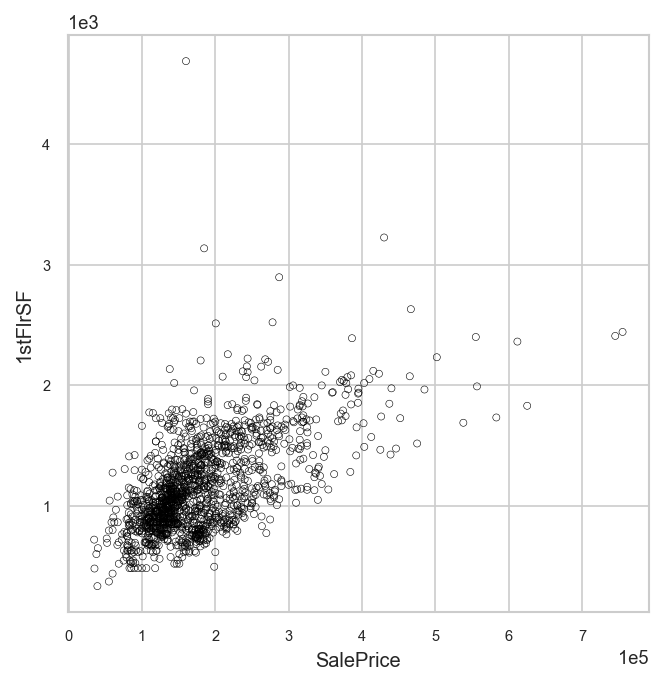
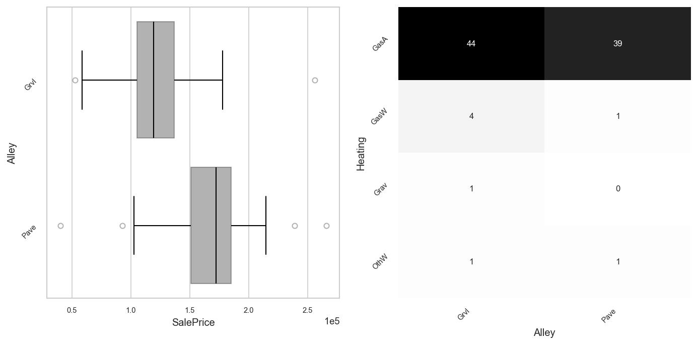
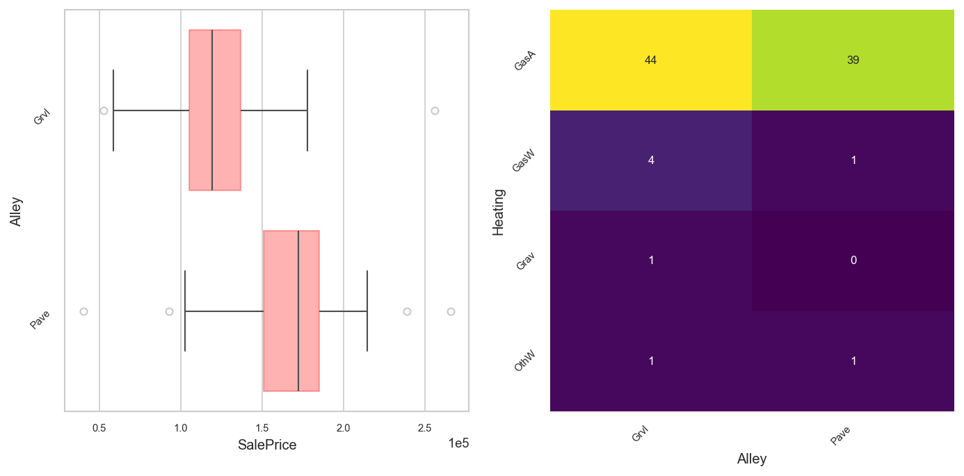
You can plot any two variables agains each other, regardless of whether they are numeric or categorical.
[11]:
fig, axs = plt.subplots(ncols=2, figsize=(11, 5))
analyzer.eda().plot("SalePrice", "Alley", ax=axs[0])
analyzer.eda().plot("Alley", "Heating", ax=axs[1])
[11]:
You can change colors.
[12]:
tm.options.plot_options.set_color_map("viridis")
tm.options.plot_options.set_bar_color("red")
fig, axs = plt.subplots(ncols=2, figsize=(11, 5))
analyzer.eda().plot("SalePrice", "Alley", ax=axs[0])
analyzer.eda().plot("Alley", "Heating", ax=axs[1])
[12]:
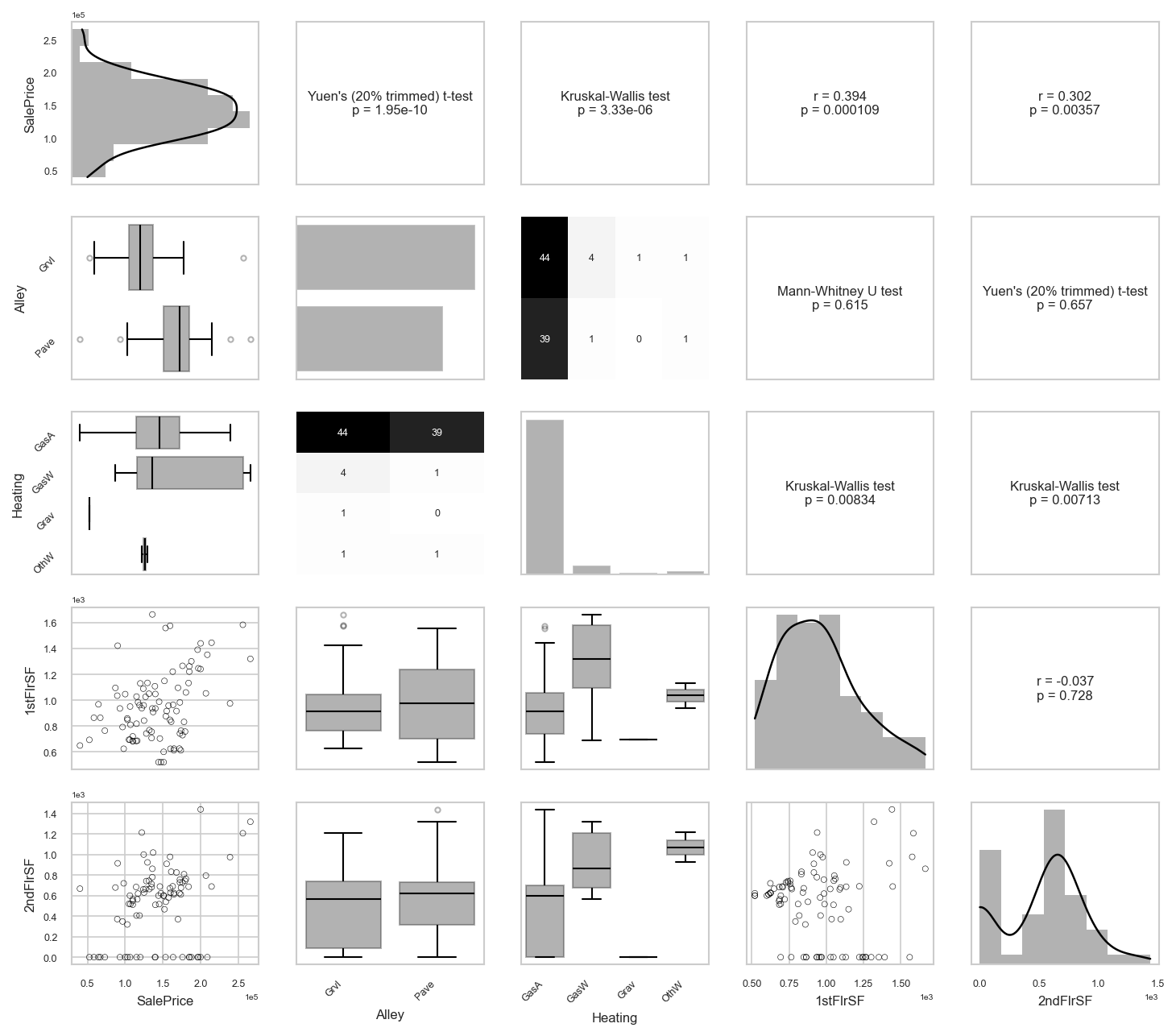
You can make pair plots, like in R. Hypothesis tests are automatically selected based on data normality and homoskedasticity
[13]:
tm.options.plot_options.set_to_defaults()
tm.options.plot_options.set_font_sizes(
    axis_title=8, major_ticklabel=6, minor_ticklabel=5
)
analyzer.eda().plot_pairs(
    ["SalePrice", "Alley", "Heating", "1stFlrSF", "2ndFlrSF"],
    htest=True,
    figsize=(10, 10),
)
[13]:
2.2 Tables
We can display all the basic statistics of each numerical variable.
[14]:
analyzer.eda().numeric_stats()
[14]:
| Statistic | min | max | mean | std | variance | skew | kurtosis | q1 | median | q3 | n_missing | missing_rate | n |
|---|---|---|---|---|---|---|---|---|---|---|---|---|---|
| Variable | |||||||||||||
| 1stFlrSF | 334.0 | 4692.0 | 1162.627 | 386.588 | 1.494501e+05 | 1.375 | 5.722 | 882.00 | 1087.0 | 1391.25 | 0 | 0.000 | 1460 |
| 2ndFlrSF | 0.0 | 2065.0 | 346.992 | 436.528 | 1.905571e+05 | 0.812 | -0.556 | 0.00 | 0.0 | 728.00 | 0 | 0.000 | 1460 |
| 3SsnPorch | 0.0 | 508.0 | 3.410 | 29.317 | 8.595060e+02 | 10.294 | 123.235 | 0.00 | 0.0 | 0.00 | 0 | 0.000 | 1460 |
| BedroomAbvGr | 0.0 | 8.0 | 2.866 | 0.816 | 6.650000e-01 | 0.212 | 2.219 | 2.00 | 3.0 | 3.00 | 0 | 0.000 | 1460 |
| BsmtFinSF1 | 0.0 | 5644.0 | 443.640 | 456.098 | 2.080255e+05 | 1.684 | 11.076 | 0.00 | 383.5 | 712.25 | 0 | 0.000 | 1460 |
| BsmtFinSF2 | 0.0 | 1474.0 | 46.549 | 161.319 | 2.602391e+04 | 4.251 | 20.040 | 0.00 | 0.0 | 0.00 | 0 | 0.000 | 1460 |
| BsmtFullBath | 0.0 | 3.0 | 0.425 | 0.519 | 2.690000e-01 | 0.595 | -0.840 | 0.00 | 0.0 | 1.00 | 0 | 0.000 | 1460 |
| BsmtHalfBath | 0.0 | 2.0 | 0.058 | 0.239 | 5.700000e-02 | 4.099 | 16.336 | 0.00 | 0.0 | 0.00 | 0 | 0.000 | 1460 |
| BsmtUnfSF | 0.0 | 2336.0 | 567.240 | 441.867 | 1.952464e+05 | 0.919 | 0.469 | 223.00 | 477.5 | 808.00 | 0 | 0.000 | 1460 |
| EnclosedPorch | 0.0 | 552.0 | 21.954 | 61.119 | 3.735550e+03 | 3.087 | 10.391 | 0.00 | 0.0 | 0.00 | 0 | 0.000 | 1460 |
| Fireplaces | 0.0 | 3.0 | 0.613 | 0.645 | 4.160000e-01 | 0.649 | -0.221 | 0.00 | 1.0 | 1.00 | 0 | 0.000 | 1460 |
| FullBath | 0.0 | 3.0 | 1.565 | 0.551 | 3.040000e-01 | 0.037 | -0.858 | 1.00 | 2.0 | 2.00 | 0 | 0.000 | 1460 |
| GarageArea | 0.0 | 1418.0 | 472.980 | 213.805 | 4.571251e+04 | 0.180 | 0.910 | 334.50 | 480.0 | 576.00 | 0 | 0.000 | 1460 |
| GarageCars | 0.0 | 4.0 | 1.767 | 0.747 | 5.580000e-01 | -0.342 | 0.216 | 1.00 | 2.0 | 2.00 | 0 | 0.000 | 1460 |
| GarageYrBlt | 1900.0 | 2010.0 | 1978.506 | 24.690 | 6.095830e+02 | -0.649 | -0.421 | 1961.00 | 1980.0 | 2002.00 | 81 | 0.055 | 1460 |
| GrLivArea | 334.0 | 5642.0 | 1515.464 | 525.480 | 2.761296e+05 | 1.365 | 4.874 | 1129.50 | 1464.0 | 1776.75 | 0 | 0.000 | 1460 |
| HalfBath | 0.0 | 2.0 | 0.383 | 0.503 | 2.530000e-01 | 0.675 | -1.077 | 0.00 | 0.0 | 1.00 | 0 | 0.000 | 1460 |
| KitchenAbvGr | 0.0 | 3.0 | 1.047 | 0.220 | 4.900000e-02 | 4.484 | 21.455 | 1.00 | 1.0 | 1.00 | 0 | 0.000 | 1460 |
| LotArea | 1300.0 | 215245.0 | 10516.828 | 9981.265 | 9.962565e+07 | 12.195 | 202.544 | 7553.50 | 9478.5 | 11601.50 | 0 | 0.000 | 1460 |
| LotFrontage | 21.0 | 313.0 | 70.050 | 24.285 | 5.897490e+02 | 2.161 | 17.375 | 59.00 | 69.0 | 80.00 | 259 | 0.177 | 1460 |
| LowQualFinSF | 0.0 | 572.0 | 5.845 | 48.623 | 2.364204e+03 | 9.002 | 82.946 | 0.00 | 0.0 | 0.00 | 0 | 0.000 | 1460 |
| MSSubClass | 20.0 | 190.0 | 56.897 | 42.301 | 1.789338e+03 | 1.406 | 1.571 | 20.00 | 50.0 | 70.00 | 0 | 0.000 | 1460 |
| MasVnrArea | 0.0 | 1600.0 | 103.685 | 181.066 | 3.278497e+04 | 2.666 | 10.044 | 0.00 | 0.0 | 166.00 | 8 | 0.005 | 1460 |
| MiscVal | 0.0 | 15500.0 | 43.489 | 496.123 | 2.461381e+05 | 24.452 | 698.601 | 0.00 | 0.0 | 0.00 | 0 | 0.000 | 1460 |
| MoSold | 1.0 | 12.0 | 6.322 | 2.704 | 7.310000e+00 | 0.212 | -0.407 | 5.00 | 6.0 | 8.00 | 0 | 0.000 | 1460 |
| OpenPorchSF | 0.0 | 547.0 | 46.660 | 66.256 | 4.389861e+03 | 2.362 | 8.457 | 0.00 | 25.0 | 68.00 | 0 | 0.000 | 1460 |
| OverallCond | 1.0 | 9.0 | 5.575 | 1.113 | 1.238000e+00 | 0.692 | 1.099 | 5.00 | 5.0 | 6.00 | 0 | 0.000 | 1460 |
| OverallQual | 1.0 | 10.0 | 6.099 | 1.383 | 1.913000e+00 | 0.217 | 0.092 | 5.00 | 6.0 | 7.00 | 0 | 0.000 | 1460 |
| PoolArea | 0.0 | 738.0 | 2.759 | 40.177 | 1.614216e+03 | 14.813 | 222.501 | 0.00 | 0.0 | 0.00 | 0 | 0.000 | 1460 |
| SalePrice | 34900.0 | 755000.0 | 180921.196 | 79442.503 | 6.311111e+09 | 1.881 | 6.510 | 129975.00 | 163000.0 | 214000.00 | 0 | 0.000 | 1460 |
| ScreenPorch | 0.0 | 480.0 | 15.061 | 55.757 | 3.108889e+03 | 4.118 | 18.372 | 0.00 | 0.0 | 0.00 | 0 | 0.000 | 1460 |
| TotRmsAbvGrd | 2.0 | 14.0 | 6.518 | 1.625 | 2.642000e+00 | 0.676 | 0.874 | 5.00 | 6.0 | 7.00 | 0 | 0.000 | 1460 |
| TotalBsmtSF | 0.0 | 6110.0 | 1057.429 | 438.705 | 1.924624e+05 | 1.523 | 13.201 | 795.75 | 991.5 | 1298.25 | 0 | 0.000 | 1460 |
| WoodDeckSF | 0.0 | 857.0 | 94.245 | 125.339 | 1.570981e+04 | 1.540 | 2.979 | 0.00 | 0.0 | 168.00 | 0 | 0.000 | 1460 |
| YearBuilt | 1872.0 | 2010.0 | 1971.268 | 30.203 | 9.122150e+02 | -0.613 | -0.442 | 1954.00 | 1973.0 | 2000.00 | 0 | 0.000 | 1460 |
| YearRemodAdd | 1950.0 | 2010.0 | 1984.866 | 20.645 | 4.262330e+02 | -0.503 | -1.272 | 1967.00 | 1994.0 | 2004.00 | 0 | 0.000 | 1460 |
| YrSold | 2006.0 | 2010.0 | 2007.816 | 1.328 | 1.764000e+00 | 0.096 | -1.191 | 2007.00 | 2008.0 | 2009.00 | 0 | 0.000 | 1460 |
We can also list out all the statistics for categorical variables.
[15]:
analyzer.eda().categorical_stats()
[15]:
| Statistic | n_unique | most_common | least_common | n_missing | missing_rate | n |
|---|---|---|---|---|---|---|
| Variable | ||||||
| Alley | 2 | Grvl | Pave | 1369 | 0.937671 | 1460 |
| BldgType | 5 | 1Fam | 2fmCon | 0 | 0.0 | 1460 |
| BsmtCond | 4 | TA | Po | 37 | 0.025342 | 1460 |
| BsmtExposure | 4 | No | Mn | 38 | 0.026027 | 1460 |
| BsmtFinType1 | 6 | Unf | LwQ | 37 | 0.025342 | 1460 |
| BsmtFinType2 | 6 | Unf | GLQ | 38 | 0.026027 | 1460 |
| BsmtQual | 4 | TA | Fa | 37 | 0.025342 | 1460 |
| CentralAir | 2 | Y | N | 0 | 0.0 | 1460 |
| Condition1 | 9 | Norm | RRNe | 0 | 0.0 | 1460 |
| Condition2 | 8 | Norm | PosA | 0 | 0.0 | 1460 |
| Electrical | 5 | SBrkr | Mix | 1 | 0.000685 | 1460 |
| ExterCond | 5 | TA | Po | 0 | 0.0 | 1460 |
| ExterQual | 4 | TA | Fa | 0 | 0.0 | 1460 |
| Exterior1st | 15 | VinylSd | ImStucc | 0 | 0.0 | 1460 |
| Exterior2nd | 16 | VinylSd | Other | 0 | 0.0 | 1460 |
| Fence | 4 | MnPrv | MnWw | 1179 | 0.807534 | 1460 |
| FireplaceQu | 5 | Gd | Po | 690 | 0.472603 | 1460 |
| Foundation | 6 | PConc | Wood | 0 | 0.0 | 1460 |
| Functional | 7 | Typ | Sev | 0 | 0.0 | 1460 |
| GarageCond | 5 | TA | Ex | 81 | 0.055479 | 1460 |
| GarageFinish | 3 | Unf | Fin | 81 | 0.055479 | 1460 |
| GarageQual | 5 | TA | Po | 81 | 0.055479 | 1460 |
| GarageType | 6 | Attchd | 2Types | 81 | 0.055479 | 1460 |
| Heating | 6 | GasA | Floor | 0 | 0.0 | 1460 |
| HeatingQC | 5 | Ex | Po | 0 | 0.0 | 1460 |
| HouseStyle | 8 | 1Story | 2.5Fin | 0 | 0.0 | 1460 |
| KitchenQual | 4 | TA | Fa | 0 | 0.0 | 1460 |
| LandContour | 4 | Lvl | Low | 0 | 0.0 | 1460 |
| LandSlope | 3 | Gtl | Sev | 0 | 0.0 | 1460 |
| LotConfig | 5 | Inside | FR3 | 0 | 0.0 | 1460 |
| LotShape | 4 | Reg | IR3 | 0 | 0.0 | 1460 |
| MSZoning | 5 | RL | C (all) | 0 | 0.0 | 1460 |
| MasVnrType | 3 | BrkFace | BrkCmn | 872 | 0.59726 | 1460 |
| MiscFeature | 4 | Shed | TenC | 1406 | 0.963014 | 1460 |
| Neighborhood | 25 | NAmes | Blueste | 0 | 0.0 | 1460 |
| PavedDrive | 3 | Y | P | 0 | 0.0 | 1460 |
| PoolQC | 3 | Gd | Fa | 1453 | 0.995205 | 1460 |
| RoofMatl | 8 | CompShg | Metal | 0 | 0.0 | 1460 |
| RoofStyle | 6 | Gable | Shed | 0 | 0.0 | 1460 |
| SaleCondition | 6 | Normal | AdjLand | 0 | 0.0 | 1460 |
| SaleType | 9 | WD | Con | 0 | 0.0 | 1460 |
| Street | 2 | Pave | Grvl | 0 | 0.0 | 1460 |
| Utilities | 2 | AllPub | NoSeWa | 0 | 0.0 | 1460 |
We can compute the correlation matrix for a set of numeric variables.
[16]:
analyzer.eda().tabulate_correlation_matrix(
    ["SalePrice", "1stFlrSF", "2ndFlrSF", "YrSold"], htest=True
)
[16]:
| SalePrice | 1stFlrSF | 2ndFlrSF | YrSold | |
|---|---|---|---|---|
| SalePrice | 1.000 (1.000) | 0.606 (0.000) | 0.319 (0.000) | -0.029 (0.269) |
| 1stFlrSF | 0.606 (0.000) | 1.000 (1.000) | -0.203 (0.000) | -0.014 (0.603) |
| 2ndFlrSF | 0.319 (0.000) | -0.203 (0.000) | 1.000 (1.000) | -0.029 (0.273) |
| YrSold | -0.029 (0.269) | -0.014 (0.603) | -0.029 (0.273) | 1.000 (1.000) |
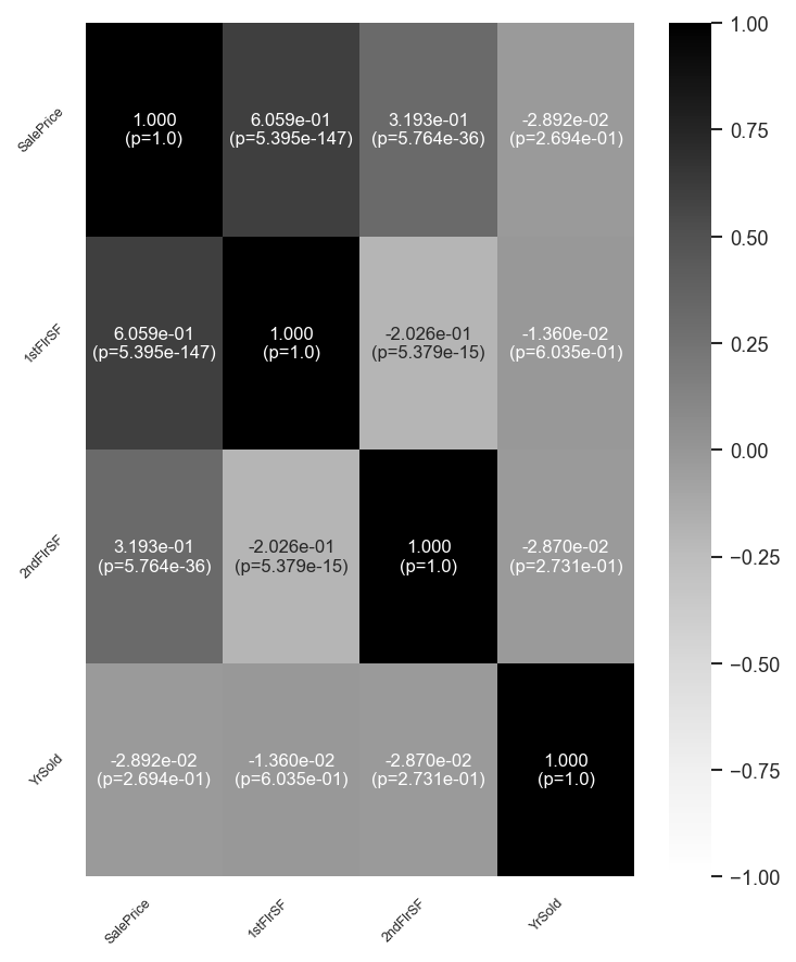
Here’s the same thing as a figure.
[17]:
analyzer.eda().plot_correlation_heatmap(
    ["SalePrice", "1stFlrSF", "2ndFlrSF", "YrSold"], htest=True, figsize=(5, 6)
)
[17]:
Correlations can be compared between a set of numeric variables and a specific numeric variable of interest. Here, we are interested in how square footage and year sold correlate with sale price.
[18]:
analyzer.eda().tabulate_correlation_comparison(
    numeric_vars=["1stFlrSF", "2ndFlrSF", "YrSold"],
    target="SalePrice",
    bonferroni_correction=True,
)
[18]:
| Corr. w SalePrice | p-value (Bonferroni corrected) | |
|---|---|---|
| 1stFlrSF | 0.606 | 1.618e-146 |
| 2ndFlrSF | 0.319 | 1.729e-35 |
| YrSold | -0.029 | 8.082e-01 |
We leverage the Python tableone package to make descriptive exploratory tables.
[19]:
analyzer.eda().tabulate_tableone(
    vars=["SalePrice", "1stFlrSF", "2ndFlrSF", "YrSold", "BldgType"],
    stratify_by="GarageFinish",
)
[19]:
| Grouped by GarageFinish | ||||||||
|---|---|---|---|---|---|---|---|---|
| Missing | Overall | Fin | RFn | Unf | P-Value | Test | ||
| n | 1460 | 352 | 422 | 605 | ||||
| SalePrice, mean (SD) | 0 | 180921.2 (79442.5) | 240052.7 (96960.6) | 202068.9 (63536.2) | 142156.4 (46498.5) | <0.001 | One-way ANOVA | |
| 1stFlrSF, mean (SD) | 0 | 1162.6 (386.6) | 1326.5 (479.3) | 1240.6 (351.5) | 1046.0 (298.4) | <0.001 | One-way ANOVA | |
| 2ndFlrSF, mean (SD) | 0 | 347.0 (436.5) | 452.3 (503.3) | 341.1 (448.2) | 304.5 (381.3) | <0.001 | One-way ANOVA | |
| YrSold, n (%) | 2006 | 314 (21.5) | 74 (21.0) | 92 (21.8) | 133 (22.0) | 0.997 | Chi-squared | |
| 2007 | 329 (22.5) | 79 (22.4) | 93 (22.0) | 140 (23.1) | ||||
| 2008 | 304 (20.8) | 74 (21.0) | 89 (21.1) | 118 (19.5) | ||||
| 2009 | 338 (23.2) | 85 (24.1) | 95 (22.5) | 143 (23.6) | ||||
| 2010 | 175 (12.0) | 40 (11.4) | 53 (12.6) | 71 (11.7) | ||||
| BldgType, n (%) | 1Fam | 1220 (83.6) | 296 (84.1) | 365 (86.5) | 505 (83.5) | <0.001 | Chi-squared | |
| 2fmCon | 31 (2.1) | 3 (0.9) | 2 (0.5) | 17 (2.8) | ||||
| Duplex | 52 (3.6) | 2 (0.6) | 1 (0.2) | 37 (6.1) | ||||
| Twnhs | 43 (2.9) | 2 (0.6) | 8 (1.9) | 28 (4.6) | ||||
| TwnhsE | 114 (7.8) | 49 (13.9) | 46 (10.9) | 18 (3.0) | ||||
Section 3: Regression Analysis
TableMage accelerates regression analyses. Let’s start with a basic example on the house prices dataset.
[20]:
data_path = curr_dir / "demo" / "regression" / "house_price_data" / "data.csv"
df = pd.read_csv(data_path, index_col=0)
analyzer = tm.Analyzer(
    df, test_size=0.2, split_seed=42, verbose=True, name="House Prices"
)
analyzer
[20]:
========================================================================================
House Prices
----------------------------------------------------------------------------------------
Train shape: (1168, 80)                      Test shape: (292, 80)
----------------------------------------------------------------------------------------
Categorical variables:
  'Alley', 'BldgType', 'BsmtCond', 'BsmtExposure', 'BsmtFinType1', 'BsmtFinType2',
  'BsmtQual', 'CentralAir', 'Condition1', 'Condition2', 'Electrical', 'ExterCond',
  'ExterQual', 'Exterior1st', 'Exterior2nd', 'Fence', 'FireplaceQu', 'Foundation',
  'Functional', 'GarageCond', 'GarageFinish', 'GarageQual', 'GarageType', 'Heating',
  'HeatingQC', 'HouseStyle', 'KitchenQual', 'LandContour', 'LandSlope', 'LotConfig',
  'LotShape', 'MSZoning', 'MasVnrType', 'MiscFeature', 'Neighborhood', 'PavedDrive',
  'PoolQC', 'RoofMatl', 'RoofStyle', 'SaleCondition', 'SaleType', 'Street', 'Utilities'

Numeric variables:
  '1stFlrSF', '2ndFlrSF', '3SsnPorch', 'BedroomAbvGr', 'BsmtFinSF1', 'BsmtFinSF2',
  'BsmtFullBath', 'BsmtHalfBath', 'BsmtUnfSF', 'EnclosedPorch', 'Fireplaces',
  'FullBath', 'GarageArea', 'GarageCars', 'GarageYrBlt', 'GrLivArea', 'HalfBath',
  'KitchenAbvGr', 'LotArea', 'LotFrontage', 'LowQualFinSF', 'MSSubClass', 'MasVnrArea',
  'MiscVal', 'MoSold', 'OpenPorchSF', 'OverallCond', 'OverallQual', 'PoolArea',
  'SalePrice', 'ScreenPorch', 'TotRmsAbvGrd', 'TotalBsmtSF', 'WoodDeckSF', 'YearBuilt',
  'YearRemodAdd', 'YrSold'
========================================================================================
Let’s first preprocess the data some.
[21]:
analyzer.dropna(include_vars=["SalePrice"]).impute(
    include_vars=["1stFlrSF", "2ndFlrSF", "YrSold"]
)
[21]:
========================================================================================
House Prices
----------------------------------------------------------------------------------------
Train shape: (1168, 80)                      Test shape: (292, 80)
----------------------------------------------------------------------------------------
Categorical variables:
  'Alley', 'BldgType', 'BsmtCond', 'BsmtExposure', 'BsmtFinType1', 'BsmtFinType2',
  'BsmtQual', 'CentralAir', 'Condition1', 'Condition2', 'Electrical', 'ExterCond',
  'ExterQual', 'Exterior1st', 'Exterior2nd', 'Fence', 'FireplaceQu', 'Foundation',
  'Functional', 'GarageCond', 'GarageFinish', 'GarageQual', 'GarageType', 'Heating',
  'HeatingQC', 'HouseStyle', 'KitchenQual', 'LandContour', 'LandSlope', 'LotConfig',
  'LotShape', 'MSZoning', 'MasVnrType', 'MiscFeature', 'Neighborhood', 'PavedDrive',
  'PoolQC', 'RoofMatl', 'RoofStyle', 'SaleCondition', 'SaleType', 'Street', 'Utilities'

Numeric variables:
  '1stFlrSF', '2ndFlrSF', '3SsnPorch', 'BedroomAbvGr', 'BsmtFinSF1', 'BsmtFinSF2',
  'BsmtFullBath', 'BsmtHalfBath', 'BsmtUnfSF', 'EnclosedPorch', 'Fireplaces',
  'FullBath', 'GarageArea', 'GarageCars', 'GarageYrBlt', 'GrLivArea', 'HalfBath',
  'KitchenAbvGr', 'LotArea', 'LotFrontage', 'LowQualFinSF', 'MSSubClass', 'MasVnrArea',
  'MiscVal', 'MoSold', 'OpenPorchSF', 'OverallCond', 'OverallQual', 'PoolArea',
  'SalePrice', 'ScreenPorch', 'TotRmsAbvGrd', 'TotalBsmtSF', 'WoodDeckSF', 'YearBuilt',
  'YearRemodAdd', 'YrSold'
========================================================================================
It’s really easy to fit an OLS model.
[22]:
report = analyzer.ols(target="SalePrice", predictors=["1stFlrSF", "2ndFlrSF", "YrSold"])
report
[22]:
========================================================================================
Ordinary Least Squares Regression Report
----------------------------------------------------------------------------------------
Target variable:
  'SalePrice'

Predictor variables (3):
  '1stFlrSF', '2ndFlrSF', 'YrSold'
----------------------------------------------------------------------------------------
Metrics:
  Train (1168)                               Test (292)
    R2:       0.548                            R2:       0.636
    Adj. R2:  0.547                            Adj. R2:  0.633
    RMSE:     51925.911                        RMSE:     52810.739
----------------------------------------------------------------------------------------
Coefficients:
                            Estimate         Std. Error            p-value
  Predictor
  const                  -876198.651        2181846.129              0.688
  1stFlrSF                   137.096             15.182              0.000
  2ndFlrSF                    80.969              6.990              0.000
  YrSold                     432.707           1086.173              0.690
========================================================================================
[23]:
report.metrics(dataset="both")
[23]:
| OLS Linear Model | ||
|---|---|---|
| Dataset | Statistic | |
| train | rmse | 51925.911 |
| mae | 34482.403 | |
| mape | 0.205 | |
| pearsonr | 0.740 | |
| spearmanr | 0.771 | |
| r2 | 0.548 | |
| adjr2 | 0.547 | |
| n_obs | 1168.000 | |
| test | rmse | 52810.739 |
| mae | 35310.444 | |
| mape | 0.212 | |
| pearsonr | 0.813 | |
| spearmanr | 0.806 | |
| r2 | 0.636 | |
| adjr2 | 0.633 | |
| n_obs | 292.000 |
[24]:
report.coefs(format="coef(se)|pval")
[24]:
| Estimate (Std. Error) | p-value | |
|---|---|---|
| const | -876198.651 (2181846.129) | 0.688 |
| 1stFlrSF | 137.096 (15.182) | 0.000 |
| 2ndFlrSF | 80.969 (6.99) | 0.000 |
| YrSold | 432.707 (1086.173) | 0.690 |
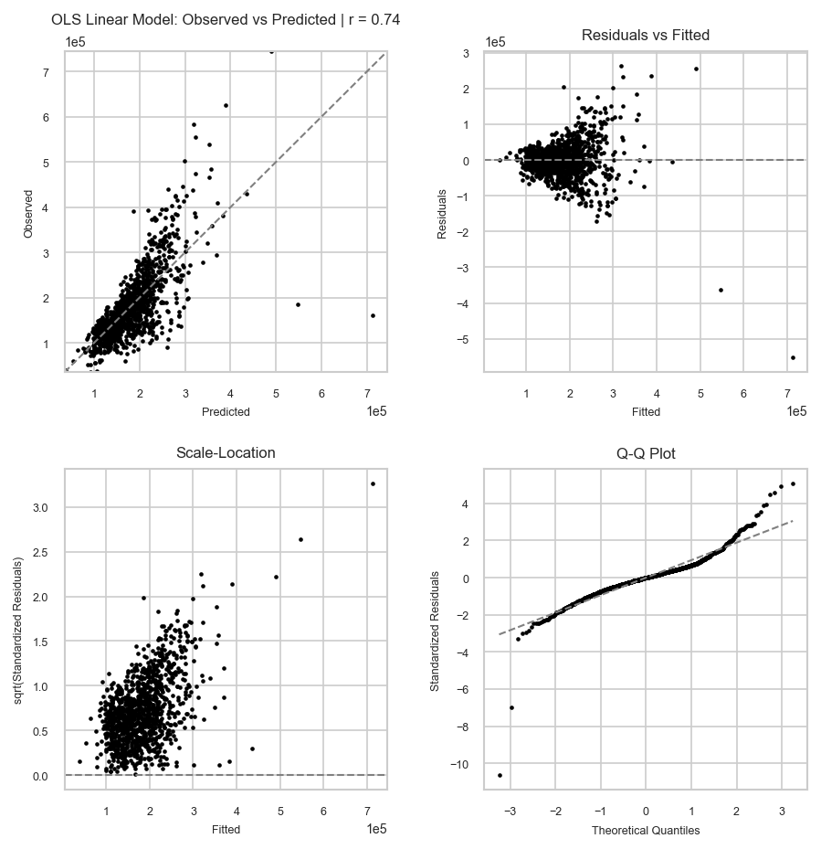
[25]:
report.plot_diagnostics("train")
[25]:
Section 4: Causal Inference
In this section, we use the TableMage package to estimate the causal effect of education on wage using a labor market dataset.
First, we load the datsaset, as shown below.
[26]:
data_path = curr_dir / "demo" / "causal" / "data" / "card.csv"
df_causal = pd.read_csv(data_path, index_col=0)
Next, we initialize an Analyzer.
[27]:
analyzer = tm.Analyzer(
    df_causal, test_size=0.2, split_seed=42, verbose=True, name="Labor Market Behavior"
)
analyzer
[27]:
========================================================================================
Labor Market Behavior
----------------------------------------------------------------------------------------
Train shape: (2408, 34)                      Test shape: (602, 34)
----------------------------------------------------------------------------------------
Categorical variables:
  None

Numeric variables:
  'IQ', 'KWW', 'age', 'black', 'educ', 'educ_binary', 'enroll', 'exper', 'expersq',
  'fatheduc', 'libcrd14', 'lwage', 'married', 'momdad14', 'motheduc', 'nearc2',
  'nearc4', 'reg661', 'reg662', 'reg663', 'reg664', 'reg665', 'reg666', 'reg667',
  'reg668', 'reg669', 'sinmom14', 'smsa', 'smsa66', 'south', 'south66', 'step14',
  'wage', 'weight'
========================================================================================
We can now make a basic causal inference model.
[28]:
causal_model = analyzer.causal(
    treatment="educ_binary",
    outcome="lwage",
    confounders=[
        "exper",
        "expersq",
        "black",
        "smsa",
        "south",
        "smsa66",
        "reg662",
        "reg663",
        "reg664",
        "reg665",
        "reg666",
        "reg667",
        "reg668",
        "reg669",
    ],
)
We can compute the difference in means naively.
[29]:
report = causal_model.estimate_ate(method="naive")
report
[29]:
========================================================================================
Causal Effect Estimation Report
----------------------------------------------------------------------------------------
Estimate: 0.194                             Std Err: 0.016
Estimand: Avg Trmt Effect (ATE)             p-value: 0.000e+00
----------------------------------------------------------------------------------------
Treatment variable:
  'educ_binary'

Outcome variable:
  'lwage'

Confounders:
  'exper', 'expersq', 'black', 'smsa', 'south', 'smsa66', 'reg662', 'reg663', 'reg664',
  'reg665', 'reg666', 'reg667', 'reg668', 'reg669'
----------------------------------------------------------------------------------------
Method:
  Naive Estimator (Difference in Means)
========================================================================================
With the introduction of these cofounders, we should estimate the ATE with a method that takes confounding into account. Let’s use outcome regression.
[30]:
report = causal_model.estimate_ate(method="outcome_regression", robust_se="nonrobust")
report
[30]:
========================================================================================
Causal Effect Estimation Report
----------------------------------------------------------------------------------------
Estimate: 0.238                             Std Err: 0.017
Estimand: Avg Trmt Effect (ATE)             p-value: 5.107e-42
----------------------------------------------------------------------------------------
Treatment variable:
  'educ_binary'

Outcome variable:
  'lwage'

Confounders:
  'exper', 'expersq', 'black', 'smsa', 'south', 'smsa66', 'reg662', 'reg663', 'reg664',
  'reg665', 'reg666', 'reg667', 'reg668', 'reg669'
----------------------------------------------------------------------------------------
Method:
  Outcome Regression
========================================================================================
Here’s another example where we apply the IPW (inverse probability weighting) estimator to estimate the ATT (average treatment effect on the treated).
[31]:
report = causal_model.estimate_att(method="ipw_weighted_regression", robust_se="HC0")
report
[31]:
========================================================================================
Causal Effect Estimation Report
----------------------------------------------------------------------------------------
Estimate: 0.232                             Std Err: 0.020
Estimand: Avg Trmt Effect on Trtd (ATT)     p-value: 2.192e-31
----------------------------------------------------------------------------------------
Treatment variable:
  'educ_binary'

Outcome variable:
  'lwage'

Confounders:
  'exper', 'expersq', 'black', 'smsa', 'south', 'smsa66', 'reg662', 'reg663', 'reg664',
  'reg665', 'reg666', 'reg667', 'reg668', 'reg669'
----------------------------------------------------------------------------------------
Method:
  Inverse Probability Weighting (IPW) Weighted Regression
========================================================================================
Section 5: Machine Learning
Now, let’s work through how to do machine learning model benchmarking using TableMage.
To begin, let’s use the house price data once again.
[32]:
import joblib
import numpy as np

data_path = curr_dir / "demo" / "regression" / "house_price_data" / "data.csv"
df = pd.read_csv(data_path, index_col=0)
analyzer = tm.Analyzer(
    df, test_size=0.2, split_seed=42, verbose=True, name="House Prices"
)
analyzer
[32]:
========================================================================================
House Prices
----------------------------------------------------------------------------------------
Train shape: (1168, 80)                      Test shape: (292, 80)
----------------------------------------------------------------------------------------
Categorical variables:
  'Alley', 'BldgType', 'BsmtCond', 'BsmtExposure', 'BsmtFinType1', 'BsmtFinType2',
  'BsmtQual', 'CentralAir', 'Condition1', 'Condition2', 'Electrical', 'ExterCond',
  'ExterQual', 'Exterior1st', 'Exterior2nd', 'Fence', 'FireplaceQu', 'Foundation',
  'Functional', 'GarageCond', 'GarageFinish', 'GarageQual', 'GarageType', 'Heating',
  'HeatingQC', 'HouseStyle', 'KitchenQual', 'LandContour', 'LandSlope', 'LotConfig',
  'LotShape', 'MSZoning', 'MasVnrType', 'MiscFeature', 'Neighborhood', 'PavedDrive',
  'PoolQC', 'RoofMatl', 'RoofStyle', 'SaleCondition', 'SaleType', 'Street', 'Utilities'

Numeric variables:
  '1stFlrSF', '2ndFlrSF', '3SsnPorch', 'BedroomAbvGr', 'BsmtFinSF1', 'BsmtFinSF2',
  'BsmtFullBath', 'BsmtHalfBath', 'BsmtUnfSF', 'EnclosedPorch', 'Fireplaces',
  'FullBath', 'GarageArea', 'GarageCars', 'GarageYrBlt', 'GrLivArea', 'HalfBath',
  'KitchenAbvGr', 'LotArea', 'LotFrontage', 'LowQualFinSF', 'MSSubClass', 'MasVnrArea',
  'MiscVal', 'MoSold', 'OpenPorchSF', 'OverallCond', 'OverallQual', 'PoolArea',
  'SalePrice', 'ScreenPorch', 'TotRmsAbvGrd', 'TotalBsmtSF', 'WoodDeckSF', 'YearBuilt',
  'YearRemodAdd', 'YrSold'
========================================================================================
Feel free to perform any preprocessing steps.
[33]:
analyzer.dropna(
    include_vars=["SalePrice"]
).drop_highly_missing_vars(  # drop variables with more than 30% missing values
    exclude_vars=["SalePrice"], threshold=0.3
).impute(  # impute missing values
    exclude_vars=["SalePrice"],
    numeric_strategy="5nn",
    categorical_strategy="most_frequent",
).scale(  # scale numeric variables
    exclude_vars=["SalePrice"], strategy="standardize"
)
[33]:
========================================================================================
House Prices
----------------------------------------------------------------------------------------
Train shape: (1168, 74)                      Test shape: (292, 74)
----------------------------------------------------------------------------------------
Categorical variables:
  'BldgType', 'BsmtCond', 'BsmtExposure', 'BsmtFinType1', 'BsmtFinType2', 'BsmtQual',
  'CentralAir', 'Condition1', 'Condition2', 'Electrical', 'ExterCond', 'ExterQual',
  'Exterior1st', 'Exterior2nd', 'Foundation', 'Functional', 'GarageCond',
  'GarageFinish', 'GarageQual', 'GarageType', 'Heating', 'HeatingQC', 'HouseStyle',
  'KitchenQual', 'LandContour', 'LandSlope', 'LotConfig', 'LotShape', 'MSZoning',
  'Neighborhood', 'PavedDrive', 'RoofMatl', 'RoofStyle', 'SaleCondition', 'SaleType',
  'Street', 'Utilities'

Numeric variables:
  '1stFlrSF', '2ndFlrSF', '3SsnPorch', 'BedroomAbvGr', 'BsmtFinSF1', 'BsmtFinSF2',
  'BsmtFullBath', 'BsmtHalfBath', 'BsmtUnfSF', 'EnclosedPorch', 'Fireplaces',
  'FullBath', 'GarageArea', 'GarageCars', 'GarageYrBlt', 'GrLivArea', 'HalfBath',
  'KitchenAbvGr', 'LotArea', 'LotFrontage', 'LowQualFinSF', 'MSSubClass', 'MasVnrArea',
  'MiscVal', 'MoSold', 'OpenPorchSF', 'OverallCond', 'OverallQual', 'PoolArea',
  'SalePrice', 'ScreenPorch', 'TotRmsAbvGrd', 'TotalBsmtSF', 'WoodDeckSF', 'YearBuilt',
  'YearRemodAdd', 'YrSold'
========================================================================================
We can use the regress function in our analyzer to properly benchmark certain models. In this case, we compare the Random Forest, XGBoost, and linear regression models.
[34]:
reg_report = analyzer.regress(
    models=[
        tm.ml.LinearR("l2"),
        # tm.ml.TreesR("random_forest"),
        # tm.ml.TreesR("xgboost"),
    ],
    target="SalePrice",
    predictors=["1stFlrSF", "2ndFlrSF", "YrSold", "BldgType", "MSZoning", "LotShape"],
    feature_selectors=[tm.fs.BorutaFSR()],  # select features
)
Lastly, we can compare model metrics and save models for future use.
[35]:
# Compare model performance
display(reg_report.metrics("test"))

# Predict on new data
new_df = df.sample(frac=0.3)
new_df = new_df.drop(columns=["SalePrice"])

y_pred = reg_report.model("LinearR(l2)").sklearn_pipeline().predict(new_df)

# Save model as sklearn pipeline
joblib.dump(reg_report.model("LinearR(l2)").sklearn_pipeline(), "l2_pipeline.joblib")

# Load model and predict on new data
y_pred_from_save = joblib.load("l2_pipeline.joblib").predict(new_df)
| LinearR(l2) | |
|---|---|
| Statistic | |
| rmse | 50294.432 |
| mae | 32321.420 |
| mape | 0.194 |
| pearsonr | 0.832 |
| spearmanr | 0.861 |
| r2 | 0.670 |
| adjr2 | 0.666 |
| n_obs | 292.000 |
Section 6: Conversational Data Analysis
In this section, we demonstrate how to use TableMage’s conversational data analysis capabilities. This is particularly useful for no-code use of the package, helping those that may not have the background necessary to do thorough data analysis on their datasets.
First, we enable the use of agents in TableMage with the tm.use_agents() function.
[36]:
from IPython.display import Markdown

tm.use_agents()
We then set the API key for the OpenAI agent using the tm.agents.set_key method. We also configure the agent to use the GPT-4o model with the tm.agents.options.set_llm method.
[37]:
tm.agents.set_key(
    "openai",
    "your-api-key-here",
)
tm.agents.options.set_llm(llm_type="openai", model_name="gpt-4o")
We initialize a ChatDA agent with the training dataset df and a test size of 20%.
[38]:
agent = tm.agents.ChatDA(df=df, test_size=0.2, verbose=False)
We interact with the agent through the chat method.
[39]:
response = agent.chat("Tell me about the dataset.")
Markdown(response)
[39]:
Your dataset consists of 80 variables, with 43 being categorical and 37 being numeric. The training set contains 1,168 rows, while the test set has 292 rows.
Numeric Variables
Some of the numeric variables include:
1stFlrSF, 2ndFlrSF, 3SsnPorch: These likely represent square footage measurements for different parts of a property.
BedroomAbvGr, FullBath, HalfBath: These could indicate the number of bedrooms and bathrooms above ground.
GarageArea, GarageCars: These might represent the area of the garage and the number of cars it can accommodate.
LotArea, LotFrontage: These could be measurements related to the property’s lot size.
SalePrice: This is likely the target variable, representing the sale price of the property.
Categorical Variables
Some of the categorical variables include:
Alley, BldgType, BsmtCond: These might describe features related to the alley access, building type, and basement condition.
CentralAir, Electrical, Heating: These could indicate the presence of central air conditioning, electrical system type, and heating quality.
Neighborhood, MSZoning: These might describe the neighborhood and zoning classification.
SaleCondition, SaleType: These could relate to the conditions and types of sales.
This dataset seems to be related to real estate, possibly for predicting house prices based on various features of the properties. If you need more detailed insights, such as summary statistics or handling missing values, feel free to ask!
[40]:
response = agent.chat(
    """Provide the summary statistics.
    Also help me figure out which variables are highly correlated with SalePrice.
    """
)
Markdown(response)
[40]:
Summary Statistics
Numeric Variables
1stFlrSF: Mean = 1162.63, Std = 386.59, Min = 334, Max = 4692
2ndFlrSF: Mean = 346.99, Std = 436.53, Min = 0, Max = 2065
GrLivArea: Mean = 1515.46, Std = 525.48, Min = 334, Max = 5642
SalePrice: Mean = 180,921.20, Std = 79,442.50, Min = 34,900, Max = 755,000
Categorical Variables
Alley: Most common = Grvl, Missing rate = 93.77%
BldgType: Most common = 1Fam, No missing values
CentralAir: Most common = Y, No missing values
Neighborhood: Most common = NAmes, No missing values
Correlation with SalePrice
The following variables have a high correlation with SalePrice:
OverallQual: Correlation = 0.791
GrLivArea: Correlation = 0.709
GarageCars: Correlation = 0.640
GarageArea: Correlation = 0.623
TotalBsmtSF: Correlation = 0.614
1stFlrSF: Correlation = 0.606
FullBath: Correlation = 0.561
YearBuilt: Correlation = 0.523
These variables are likely to be significant predictors of SalePrice. If you’re planning to build a predictive model, these features could be a good starting point. Let me know if you need further analysis or assistance!
[41]:
response = agent.chat(
    """Help me predict the SalePrice with linear regression.
    Choose the predictors you think are most relevant.
    """
)
Markdown(response)
[41]:
The linear regression model using the selected predictors (OverallQual, GrLivArea, GarageCars, GarageArea, TotalBsmtSF) has been fitted to predict SalePrice. Here are the key results:
Coefficients:
OverallQual: Significant positive impact on SalePrice ($23,835 increase per unit increase in quality).
GrLivArea: Significant positive impact ($42.43 increase per square foot).
GarageCars: Positive impact, but not statistically significant.
GarageArea: Positive impact, but not statistically significant.
TotalBsmtSF: Significant positive impact ($27.5 increase per square foot).
Model Performance:
Training Set:
RMSE: $38,625
R²: 0.75
Test Set:
RMSE: $39,979
R²: 0.792
The model explains about 75% of the variance in the training set and 79.2% in the test set, indicating a good fit.
I’ve also generated diagnostic plots for further analysis. If you have any specific questions or need further analysis, feel free to ask!
[42]:
response = agent.chat(
    """Fit some machine learning models to try to obtain better predictive performance.
    Let me know which model is best and how it performs.
    Tell me also how you trained that model.
    """
)
Markdown(response)
[42]:
I fitted several machine learning models to predict SalePrice, and here’s how they performed:
Model Performance:
XGBoost:
Training Set: RMSE: $21,697, R²: 0.921
Test Set: RMSE: $31,235, R²: 0.873
Training Details: Used Optuna for hyperparameter tuning with 100 trials and 5-fold cross-validation. Best parameters included a learning rate of 0.039, 100 estimators, and a max depth of 5.
Random Forest (RF):
Training Set: RMSE: $26,615, R²: 0.881
Test Set: RMSE: $33,444, R²: 0.854
Training Details: Optuna tuning with 100 trials. Best parameters included 400 estimators, max depth of 13, and log2 for max features.
Ridge Regression:
Training Set: RMSE: $38,627, R²: 0.75
Test Set: RMSE: $39,955, R²: 0.792
Lasso Regression:
Training Set: RMSE: $38,625, R²: 0.75
Test Set: RMSE: $39,979, R²: 0.792
Best Model:
The XGBoost model performed the best with the lowest RMSE and highest R² on both the training and test sets. It was trained using a comprehensive hyperparameter search strategy, optimizing parameters like learning rate, number of estimators, and tree depth.
If you have further questions or need additional insights, feel free to ask!
We hope you enjoy TableMage.